
In a previous post, I briefly introduced Marx’s value theory. Values and prices were considered at the aggregate level without breaking the economy down into different sectors. This enabled a focus on basic macro relationships. In this post, the economy is disaggregated into several sectors. Following the ‘temporal single-system interpretation’ (TSSI), aggregate surplus value is taken to determine the average rate of profit in the economy, prior to the determination of individual prices. If free capital mobility is assumed, there is a tendency for rates of profit to equalize across sectors. This causes a divergence of prices from values in individual sectors. Nevertheless, key aggregate equalities continue to hold, and the divergence of prices from values occurs in a systematic way, according to the composition of capital in each sector. The exposition closely follows a 1999 paper by Andrew Kliman and Ted McGlone entitled, ‘A Temporal Single-system Interpretation of Marx’s Value Theory’, published in the Review of Political Economy.
Some theory
For the economy as a whole, the total value, λ, produced over a period is equal to the sum of constant capital, c, variable capital, v, and surplus value, s:
c = the sum of value advanced to acquire the means of production used up in the period
v = the sum of value advanced to employ living labor
s = the value produced by living labor in excess of variable capital
Value and prices can be expressed in terms of money or labor time. It is always possible to switch from money terms to labor-time terms and back again using the ‘monetary expression of labor time’ (MELT). It will be assumed in the present discussion that the MELT is constant, with one hour of labor time producing $1 of value.
Marx argued that the value of constant capital is simply passed on to the value of output, whereas living labor, l = v + s, produces new value. If workers are required to work longer than is necessary to reproduce their own wages and benefits (v), there will be surplus value, s = l – v, left over for the capitalist class, prior to its distribution into retained profit, interest, rent, and so on.
These value relationships continue to hold at disaggregated levels of analysis. The value magnitudes applying to an individual sector, i, will be denoted ci, vi, si, and so on.
The value, λi, of sector i’s output is equal to the amount of constant capital that is transferred to the final product(s) plus the living labor performed to produce it. For simplicity, it is assumed that all constant capital is used up – or transferred to final output – each period. More generally, only a portion of fixed capital will be passed on to the final output each period, so the simplifying assumption amounts to assuming there is no fixed capital, only circulating capital. Any machines and materials used will be completely consumed in the production period.
The value produced in sector i is:
λi = ci + vi + si
In aggregate, total value equals total price, but for individual sectors (or lower levels of disaggregation) prices will usually diverge from values. This can occur because of various influences, including monopoly, rent, and the tendency – when money capital is mobile – for the rates of profit in different sectors to equalize.
In the present discussion, competitive conditions will be assumed, so deviations of values from prices will be due to the last influence, the tendency for profit rates to converge. Investment dollars will flow out of less profitable sectors into more profitable ones, tending to push sectoral profit rates toward the economy-wide average.
The price received by sector i differs from value produced by an amount gi, which may be positive or negative:
pi = ci + vi + si + gi
This divergence causes the sector’s profit, πi, to differ from its surplus value by the same amount gi. That is, πi = si + gi. Profit refers to an amount received by the sector, whereas surplus value refers to an amount created in production:
πi = pi – (ci + vi)
si = λi – (ci + vi)
Sometimes the sum of constant capital and variable capital is referred to as the ‘cost price’, ki.
Likewise, the sector’s rate of profit received, ri, differs from the rate of profit produced, σi. The first of these measures is known as the ‘price rate of profit’. The second is the ‘value rate of profit’. Under the assumption of no fixed capital, these are:
ri = πi / (ci + vi) = (si + gi) / (ci + vi)
σi = si / (ci + vi)
Since, for the economy as a whole, total profit equals total surplus value, the sum of all gi‘s is zero. This means that the economy-wide average price rate of profit, or simply average ‘rate of profit’, r, is equal to the average value rate of profit.
The gi‘s that are consistent with all sectors receiving the average rate of profit can be determined by rearranging the second expression for ri in the equations above, and substituting the average rate of profit, r, for ri:
gi = r(ci + vi) – si
Because of the aggregate identity between profit and surplus value, and the consequent identity between the average price rate of profit and the average value rate of profit, the average rate of profit can be determined before any individual prices are known. The rate follows from a ratio of aggregate value magnitudes:
r = s / (c + v)
Temporal single-system determination of values and prices
In the TSSI, the values and prices of output in period t+1 are determined by price and value magnitudes of period t. The process is best described with matrix algebra, but can be kept very simple. It will not be necessary to do anything more complicated than multiplying or adding two matrices together, or subtracting one from the other. If any readers are unclear on these operations, they may wish to consult the short section, Basic Operations, in the Wikipedia entry on matrix algebra. Alternatively, readers can ignore the equations and focus on a simple numerical example provided in the next section.
Value magnitudes of all sectors will be represented by vectors or matrices that are denoted by bold font. For example, the vector c = [c1 c2 c3] summarizes the constant capital of sectors 1, 2 and 3. Summing the elements of the vector gets us back to the aggregate value c for the economy as a whole. The aggregate, of course, is a single number, or ‘scalar’ in matrix algebra.
Recall that constant capital is the amount of money (or its labor-time equivalent) advanced for the means of production that are used up in production over the period. In the TSSI, this sum is equal to the period t prices of the means of production multiplied by their physical or real quantities:
ct = pt A
Here, pt is a row vector and A is a square input-output matrix of physical quantities.
Similarly, variable capital is the amount paid to workers over the period, which can be considered equal to the amount workers pay, in period t prices, for a real-wage basket, b, of consumer goods multiplied by the amount of employment:
vt = pt bl
Over time, A, b and l need not be constant, and so in general will also have time subscripts. For simplicity, it is assumed that these remain unchanged over the period.
Surplus value, as the excess of living labor over variable capital, can be written:
st = l – vt = l – pt bl
In the TSSI, the vector pt is the set of prices prevailing at the moment when the means of production and labor power enter the production process. In the case of constant capital, these prices will be passed on to the final output. In the case of variable capital, the prices of the goods in the real-wage basket (or the ‘means of subsistence’) will help to determine the proportion of living labor that is necessary to reproduce the wages and benefits of the workers. This amount of labor is referred to as ‘necessary labor’. The remainder – ‘surplus labor’ – creates surplus value.
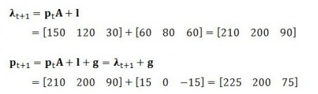
Keeping in mind that the value of output in period t+1 is equal to the sum of constant capital, variable capital and surplus value in period t, the above expressions can be substituted:
λt+1 = pt A + pt bl + (l – pt bl) = pt A + l
Differences in period t+1 between sectoral output prices and values are described by the vector gt. This enables output prices to be expressed as:
pt+1 = pt A + l + gt = λt+1 + gt
Notice that, in the TSSI, values and prices are mutually determined in a single system. On the one hand, the above expressions make clear that values in one period are determined partly by the previous period’s prices. On the other hand, it was noted earlier that value magnitudes operating at the aggregate level are determinative of prices. Specifically, total surplus value divided by cost price (c + v) determines the average rate of profit that will apply in the determination of individual output prices. It is this prior aggregate determination of the rate of profit that enables determination of the gi‘s and, therefore, individual prices.
Numerical example
The following table shows the quantities of output from each of three sectors that are used as inputs in the various production processes:
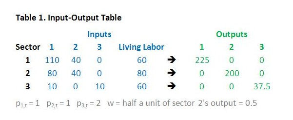
The table indicates, for instance, that sector 1 uses 110 units of its own output from period t as input for production in period t+1. It also uses 40 units of sector 2’s output and employs 60 units of labor over the period. This combination of means of production and living labor enables sector 1 to supply 225 units of output in period t+1.
The prices listed in the final row of the table are those that prevail at the time inputs enter production, which is defined to be the end of period t. The wage rate, w, is equal to half a unit of output produced in sector 2. Since the price of sector 2’s output in period t is 1, this makes the wage rate 0.5 per unit of labor.
The output quantities for the three sectors in period t+1 will be x1,t+1 = 225, x2,t+1 = 200, and x3,t+1 = 37.5.
The numbers in the input-output table can be used to calculate the values and prices that will prevail in period t+1 under the assumption that rates of profit are equalized across sectors. For instance, constant capital in sector 1 will be p1(110) + p2(40) and variable capital will be w(60). It is also assumed that the rate of exploitation, s/v, is 100%.

In sector 1, price exceeds value (225 > 210), profit exceeds surplus value (45 > 30), and the price rate of profit exceeds the value rate of profit (25% > 16.7%). The reason for this is that the composition of capital, c/v, in sector 1 is above the average (5 > 3). Investment will tend to be withdrawn or withheld from the sector sufficiently to cause the profit rate to converge on the average.
The reverse is the case in sector 3. Price magnitudes and profit rates in that sector are below their value counterparts as a result of a below-average composition of capital.
The remaining sector, sector 2, just happens to have a composition of capital equal to the aggregate composition of capital. For this reason, price and value coincide in that sector.
Notice, as anticipated, that the three aggregate identities hold. Total price equals total value, total profit equals total surplus value, and the average price rate of profit equals the average value rate of profit. With the average rate of profit determined at the aggregate level, individual prices then tend to move to the levels consistent with a uniform rate of profit across sectors.
Prices per unit of output can be calculated by dividing the sectoral prices by the physical quantities shown in the earlier, input-output table. For the first sector, the price per unit is 225/225 = 1, for the second sector 200/200 = 1, and for the third sector 75/37.5 = 2.
Although these prices for period t+1 equal the corresponding prices for period t, this need not be the case. Even without inflation, it is quite possible – in fact, likely – that the prices will change from one period to the next, due to changes in productivity. In the illustration, productivity has been treated as constant for simplicity. Inflation has also been assumed away, because it is not fundamental to the tendencies discussed.
The same example using matrix algebra
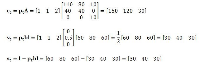
Recall that constant capital can be calculated using period t prices and the input-output information:
ct = pt A
Here, A is a square input-output matrix with three rows and three columns. These dimensions are denoted 3×3. The element in row i and column j of the matrix is denoted aij and indicates the amount of sector i’s output required by sector j for its production process. For instance, the first row of the matrix (shown below) says that 110 units of sector 1 output is required by the first sector, 80 units of sector 1 output is required by the second sector, and 10 units of sector 1 output are required by the third sector.
Similarly, variable capital and surplus value can be calculated using the appropriate vectors.
For those unfamiliar with matrix algebra, multiplication of two matrices is permissible if the number of columns of the left matrix equals the number of rows of the right matrix. If so, the resulting matrix will have the same number of rows as the left matrix and the same number of columns as the right matrix.
For instance, in the multiplication of pt A above, the left matrix is 1×3 and the right matrix is 3×3. The “inside” dimensions (3 and 3) tell us that it is okay to multiply. The “outside” dimensions (1 and 3) tell us that the result will be a 1×3 matrix.
Each element of the resulting matrix is calculated by taking the ‘inner product’ (or ‘sum product’) of a row of the left matrix and column of the right matrix. The resulting element will be positioned in the same row as the left-matrix row, and the same column as the right-matrix column.
As an example, the inner product of the first row of pt and the first column of A is 1(110) + 1(40) + 2(0). The result, 150, is in the first row and first column of the resulting matrix.
In the special case of multiplying a matrix by a single number (a ‘scalar’), simply multiply each element of the matrix by the scalar. This is done in the second row of working above, where each row of a 1×3 vector is multiplied by 1/2.
Addition or subtraction of two matrices can occur when both matrices have the same dimensions. The resulting matrix will also share these dimensions. Simply add corresponding elements together to arrive at the corresponding cell in the resulting matrix. This occurs above in the third row of working.
Before calculating the values and prices for period t+1, it can be noted that, in aggregate, constant capital, variable capital and surplus value are 300, 100 and 100, respectively. These amounts are found by summing the elements of the relevant vectors.
The economy-wide, average rate of profit, r, is s/(c+v) or 25%.
This knowledge can be used to determine the price-value deviations.
Recalling that gi = r(ci + vi) – si:
g1 = 25%(150 + 30) – 30 = 15
g2 = 25%(120 + 40) – 40 = 0
g3 = 25%(30 + 30) – 30 = –15
As required, the price-value differences sum to zero.
It is now possible to calculate the output values and prices for period t+1.
Summing the elements of the period t+1 value and price vectors indicates that total value equals total price, as required.
