This is intended as an introductory post to explain the Keynesian (and Kaleckian) view of causation between desired investment and desired saving in particular, and desired injections and desired leakages in general. Initially, the argument is presented with reference to a simple two-sector income-expenditure model of a pure private economy. The model illustrates the Keynesian view that provided the economy is operating below full employment and there is idle capacity, desired investment generates desired saving via income adjustments rather than being financed by that saving. The second part of the post employs a four-sector model with government and external sectors included to draw out a couple of points emphasized by Modern Monetary Theorists.

 
1. The two-sector income-expenditure model

In a pure private economy, the two sectors could either be workers and capitalists or households and firms. Kalecki chose the former, Keynes the latter. It doesn’t matter which is chosen for present purposes because both Kalecki and Keynes came to the same conclusions regarding causation. Here, the Keynesian version is presented.

The Keynesian models to be considered are short run in nature in that the productive capacity of the economy is taken as given. That means the effect of investment on productive capacity is abstracted from and only its impact on current demand and income is taken into account. This assumption is not as strange as it may seem, since the impact of investment on capacity lags behind its effect on current demand and income.

 
Identities

Several aggregate relationships must hold by definition:

Y = E = C + I

Y = C + S

S = I

All variables are in real (i.e. price-deflated) terms. The first identity says that income, Y, always equals total expenditure, E. Total expenditure is comprised of two types of spending: consumption, C, and investment, I. Investment is capacity-expanding expenditure such as fixed investment in plant and machinery as well as unsold inventories, since these also add to the capacity of the economy to meet demand. The second identity refers to the uses of income. It can be consumed or saved, S. The third identity indicates that saving always equals investment. It follows directly from the first two identities.

Identities do not imply equilibrium. The first and third identities hold because of the way investment is defined. Although unsold inventories are capacity-expanding and so counted as investment, the amount of inventories held by firms may be intentional or a mistake.

 
Equilibrium

Macroeconomic equilibrium requires desires (or plans) to be realized. If desires are not realized, there will be an impetus for change as firms and households attempt to bring actual outcomes into conformity with their desires.

Equilibrium only occurs if:

Y_e = E_d = C_d + I_d

S_d = I_d

The ‘e’ subscript indicates an equilibrium level. The ‘d’ subscripts indicate desired magnitudes. It is only when income or output match desired total expenditure that the economy is in equilibrium. The second equilibrium condition follows directly from the first by simple rearrangement, noting that Y – C_d = S_d.

Out of equilibrium, actual saving and investment include both desired and undesired components:

S = S_d + S_u

I = I_d + I_u

Undesired investment, I_u, refers to unexpected changes in inventories. Undesired saving, S_u, can occur when goods or services are temporarily unavailable, due to shortages or interruptions in production.

Clearly, the equilibrium conditions will only hold when actual saving and investment coincide with their desired levels:

S = S_d

I = I_d

S_u = 0 = I_u

 
Causation

Whenever desires go unrealized, there is disequilibrium. To say anything about the way the economy might move from disequilibrium to equilibrium, it is necessary to make an argument concerning causation. And this requires making behavioral assumptions. Unlike identities, behavioral assumptions are contestable.

A key assumption of the model is that firms will respond to unanticipated changes in inventories by adjusting the level of production. Many firms intentionally plan for a certain amount of inventories. These are part of desired investment and will not induce a change in behavior. But when firms sell less than anticipated, they are assumed to cut back production in an attempt to eliminate the undesired investment. In the reverse case of excess demand, inventories will be unexpectedly depleted and firms will attempt to bring negative undesired investment back up to zero by expanding production.

Desired consumption and desired saving are assumed endogenous and positively related to income, although some consumption and saving occurs independently of income. Desired investment is assumed exogenous. It is financed independently of current income out of past savings or borrowing.

The following simple model reflects these assumptions:

(A) Y_e = C_d + I_d

(B) C_d = C_o + cY

(C) I_d = I_o

The first equation is the equilibrium condition. The second and third are behavioral equations. The ‘o’ subscripts indicate exogenous variables.

In the second equation, the consumption function includes an autonomous component, C_o, and an induced component, cY, where c is the marginal propensity to consume or mpc (0 < c < 1). The mpc is the fraction of an additional increment of income that is consumed. It is assumed to be stable, at least over a realistic range of income.

Since saving is income not consumed (Y – C_d), the consumption function implies a corresponding saving function:

S_d = sY – C_o

Here, s (= 1 – c) is the marginal propensity to save or mps.

The third equation says that desired investment is exogenous or autonomous of income. This leaves the determination of investment open, making the model compatible with a variety of competing theories of investment.

Substituting the behavioral equations (B) and (C) into the equilibrium condition (A), rearranging and solving for Y yields:

This says that equilibrium income is a multiple of exogenous expenditure. The multiplier, k, is 1/(1 – c).

Suppose, for example, that:

C₀ = 0

I_d = 100

c = 0.8

From the value of the marginal propensity to consume it is clear that the multiplier is 5. Since autonomous expenditures sum to 100, equilibrium income will be 500. From this information, it is also easy to calculate desired consumption and saving:

C_d = C_o + cY = 400

S_d = sY – C_o = 100

As required, desired saving equals desired investment, and equivalently, the sum of desired consumption and desired investment equals income.

The model can be used to see how changes in the exogenous variables (autonomous consumption and desired investment) or structural parameter (the mpc) affect the endogenous variables (income, desired consumption and desired saving). Exogenous expenditure is received as income by firms and this sets in place a multiplier process as the income induces additional consumption that creates additional income. However, in each round of the process, some income leaks out to saving, so the impact of the initial exogenous expenditure becomes smaller each round until negligible. The leakages on each round of the process ensure that income (output, supply) eventually catches up to desired total expenditure (demand).

 
Example 1a. Desired investment is ‘self-financing’.

Let the economy initially be in the equilibrium described above: Y = 500, S_d = I_d = 100 and C_d = 400. Now imagine that desired investment increases from 100 to 120. The effect of this is outlined in the table below. All entries are rounded, if necessary, to whole numbers.

Round 0 shows the initial equilibrium. In round 1, the intention to increase desired investment by 20 causes excess demand as desired total expenditure outstrips income. Disequilibrium is also indicated by the undesired saving of 20.

In round 2, the injection of extra spending is received as income by firms producing investment goods and this higher income induces a response from households, who consume 80 percent of the additional income and save 20 percent, in accordance with the marginal propensities to consume and save. As a result, desired total expenditure remains above income, but by less than previously due to the leakage to saving. Notice that the increase in desired saving eliminates some of the undesired saving.

The process continues in successive rounds until equilibrium is restored. The example shows income and output adjusting to demand. Notice how income lags demand. The example also illustrates the Keynesian view of how an initial increase in desired investment that is unaccompanied by an equal intention to save nevertheless sets in motion a process by which income adjustments induce the necessary desired saving. This enables the economy to stabilize at a new, higher level of equilibrium income.

 
Example 1b. Paradox of thrift.

Let the economy start in the same initial equilibrium as in the previous example but now suppose that households decide to increase saving by 20. This can be considered an exogenous increase in saving or, equivalently, a reduction of 20 in autonomous consumption. This decision initiates the process outlined in the table below:

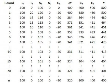
Once again, round 0 shows the initial equilibrium. In round 1, desired saving increases by 20. There is a reduction of the same amount in desired consumption due to a fall in autonomous consumption. The higher desired saving causes excess supply and undesired investment of 20.

In round 2, firms respond by cutting back production. It is assumed that in each round of the multiplier process, firms cut back by the amount of the previous round’s undesired investment. They continue to do this until undesired investment stabilizes at zero.

The example illustrates the Keynesian view of how an attempt to increase desired saving is self-defeating and cannot finance desired investment. Negative income adjustments wipe out any desired saving that is in excess of the level of desired investment.

 
2. The four-sector income-expenditure model

Introducing the government and external sectors adds two more types of expenditure: government spending, G, and exports, X. There are also two additional uses of income: taxation, T, and imports, M. These additions give rise to the following identities:

Y = C + I + G + (X – M)

Y = C + S + T

Imports are subtracted from the first identity and left out of the second to avoid double counting. In the national accounts, import spending is already included in domestic categories of expenditure.

By subtracting T from both sides of the first identity, rearranging and finally substituting S for Y – T – C, two more identities are obtained:

I + G + X = S + T + M

(S – I) + (T – G) + (M – X) = 0

The first of these shows that injections equal leakages, by definition. The second is the familiar sectoral balances identity. The financial balances of the domestic private sector, government and foreigners must cancel each other out.

Equilibrium, once again, requires desires to be realized. This condition can be stated in various equivalent ways:

Y_e = C_d + I_d + G_d + (X_d – M_d)

I_d + G_d + X_d = S_d + T_d + M_d

(S– I)_d + (T – G)* + (M – X)_d = 0

The first version of the equilibrium condition says that desired total expenditure must equal income. The second version says that desired injections must equal desired leakages. The third version says that the government’s fiscal position (T – G)* must be consistent with the desired net financial accumulation of both the domestic private sector and foreigners. The * indicates consistency with equilibrium. (See pp.17, 42 of a recent paper by Tymoigne and Wray).

In the four-sector model, government spending and exports are assumed exogenous in addition to desired investment. Taxation and imports are assumed endogenous and, like desired consumption and desired saving, positively related to income.

The following model employs these assumptions:

(1) Y_e = E_d

(2) E_d = C_d + I_d + G_d + (X_d – M_d)

(3) C_d = C_o + c(Y – T_d)

(4) T_d = T_o + tY

(5) M_d = M_o + mY

(6) I_d = I_o

(7) G_d = G_o

(8) X_d = X_o

Notice that the tax and import functions have both autonomous and induced components, similar to the consumption function. Much tax revenue is induced, but some taxes and fees are imposed independently of income. Similarly, import spending is largely connected to income but is also influenced by other factors such as the exchange rate. The parameters t and m are the marginal propensities to tax and import, respectively.

The consumption function implies the following saving function, remembering that saving is that part of disposable income not consumed (i.e. S_d = Y – T_d – C_d):

(9) S_d = s(Y – T_d) – C_o

Substituting (4) into (3), then substituting (3), (5)-(8) into the equilibrium condition, rearranging and solving for Y yields:

The numerator is net autonomous expenditure. The denominator is the reciprocal of the multiplier. The multiplier is smaller than in the two-sector model because of the additional leakages that occur due to taxes and imports during the multiplier process.

 
Example 2a. Exogenous increase in desired investment.

In calculating the following table, it was assumed that c = 0.8, s = 0.2, t = 0.25, m = 0.1. The multiplier is 2. To save space, C_o, T_o and M_o were all set to zero.

In round 0, the economy is in equilibrium, so E_d = Y and I_d + G_d + X_d = S_d + T_d + M_d. Although not necessary for equilibrium, the example starts with all sectoral budgets balanced. This was done to make the impact of the multiplier process on the three sectoral balances obvious.

In round 1, desired investment increases by 50. This causes excess demand (E_d > Y) and sets off the multiplier process.

In round 2, firms expand production to meet the higher demand. The resulting addition to income induces extra desired consumption but also leakages to saving, tax revenue and import spending. Each round, the addition to total expenditure gets smaller and income gradually adjusts to demand.

The causation is the same as in the two-sector model, but the effect of an exogenous change in demand (in this case desired investment) is felt by all leakages. The extra 50 in investment causes a multiplied change in income that eventually increases the sum of leakages by the same amount of 50. In the initial equilibrium, desired injections and leakages both summed to 500. In the new equilibrium at the higher income of 1100, desired injections and leakages both sum to 550.

Notice that the sectoral balances, which were all zero in the initial equilibrium, have diverged. The multiplied increase in income has boosted tax revenues and to a lesser extent imports. As a consequence, the government and foreigners are now in surplus by a combined amount of 35. This is offset by the domestic private sector, which is in deficit, spending more than its income.

The spending and saving behavior of the domestic private sector was such that most of the leakage created by the higher desired investment went to taxes and imports. The domestic private sector has chosen to draw down some of its accumulated financial wealth. This could go on for a while without causing problems but would eventually create an unsustainable private-debt burden if not reversed, such as occurred in the lead up to the present global financial crisis. (See Sectoral Balances and Keynesian Causation and Introduction to the Sectoral Financial Balances Model for more on this point.)

 
Example 2b. Exogenous increase in desired saving.

Whereas in the simple two-sector model a spontaneous attempt to increase desired saving is entirely self-defeating, this is not the case in the four-sector model. The negative income adjustments will now hit not only private saving but tax revenue and imports. Accordingly, the private sector can achieve higher saving to the extent that there are leakages to taxes and imports. The economic effect will still be negative if the attempt to increase saving is in isolation. There will be lower income and the government will be running a “bad deficit” in that it is caused by an endogenous reduction in tax revenue driven by falling income. If instead the government steps up its net spending to counteract the negative impact on income, the domestic private sector can have higher desired saving alongside strong income.

Referring to the table below, round 0 describes the same initial equilibrium that was in the preceding example. In round 1, the domestic private sector exogenously steps up its saving by 50. This means autonomous consumption is -50, though it is not shown in the table. For a while, the government stands by as income falls. Desired saving drops back a bit but still remains significantly above its initial level as the government’s deficit increases endogenously. Foreigners also move into deficit.

By round 9, a new equilibrium is just about reached but it is pretty awful, income having plummeted 10 percent. The domestic private sector has managed a surplus of 35, which is offset by a government deficit of 25 and external surplus of 10.

The government belatedly decides to step up its spending by 50. This sets off rounds 10-19.

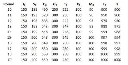
The table shows that the government has managed to offset the negative effects on income of the reduced private spending and increased saving by lifting its own expenditure. This has enabled the domestic private sector to attain its desired surplus of 50 without any decline in income.

That is not to say that the government should always simply enable the desired surplus of the domestic private sector. Private spending and saving behavior are influenced by distribution, institutional arrangements and other factors that might all need addressing.

There are various strategies that could be employed in addition to an increase in government net expenditure. A job-guarantee program could ensure full employment irrespective of the desired net financial accumulation of the domestic private sector and foreigners. A redistribution of income to middle and low-income recipients would boost activity for any given level of government expenditure. A debt jubilee would free up private income for spending that is currently devoted to private debt service. And so on.