A job guarantee would be a standing offer of a publicly funded job, with spending on the program adjusting automatically and countercyclically in response to take-up of positions. The likely feedback between spending on the program and activity in general is interesting and can be considered within the income-expenditure framework. In what follows, the standard model is modified to find the steady state levels and compositions of income and employment and other key variables. Attention then turns to how the system might behave outside a steady state. A way of conceptualizing the dynamics of the system is suggested and formulas developed to describe that behavior. The suggested dynamics are shown to be consistent with steady state requirements.
1. Income determination with a job guarantee
It will be convenient to think of the economy as comprising just two sectors: the ‘job guarantee sector’ or sector j and the ‘broader economy’ or sector b. The broader economy is taken to include households, firms, the rest of the public sector and non-residents.
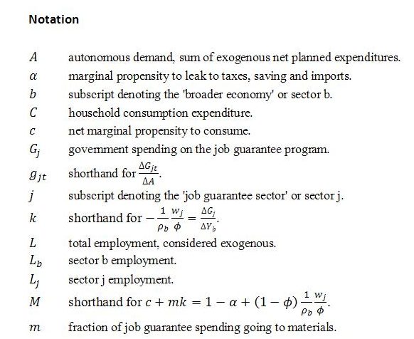
Suppose that most categories of planned expenditure are exogenous and can be lumped together as autonomous demand A. The exceptions are induced household consumption net of endogenous imports, which rises with income, and job guarantee spending, which varies countercyclically. Steady state income in the absence of a job guarantee would be A / α, where α is the marginal propensity to leak to taxes, saving and imports. With a job guarantee, the system becomes:

The first equation is the steady state condition. Income Y must equal demand Yd for activity to be stable. The second equation shows demand as the sum of induced net household consumption (1 – α)Y, autonomous demand and job guarantee spending Gj. It is assumed for simplicity that equipment and materials used in job-guarantee production are purchased from the domestic economy.
Income for the economy as a whole is composed of the sectoral incomes. The income of sector j can be regarded as the wages paid to job guarantee workers. This is in keeping with the national accounting treatment of public sector activity in general. If a fraction ϕ of job guarantee spending goes to wages, sector j income will be ϕGj. It is assumed that the remaining fraction 1 – ϕ of job guarantee spending goes on materials supplied by the broader economy and so contributes to sector b income. These considerations are summarized as:

A preliminary expression for the steady state level of total income can be obtained by solving the system of equations (1) for Y. The result can be plugged in to the third equation in (2) to give a corresponding expression for sector b income:
To progress any further, we need an expression for job guarantee spending.
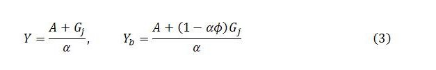
Let wj be the exogenously set job guarantee wage. With ϕ defined as the fraction of job guarantee spending going to wages, wj / ϕ must be the amount of job guarantee spending per unit of sector j employment Lj. This implies:
Sector j employment accounts for whatever employment is not located in the broader economy. This means we can write the above as

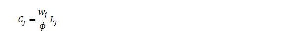
In the present discussion, total employment L is simply taken as given. This simplifying assumption means that variations in one sector’s employment translate one-for-one into inverse variations in the other sector: ΔLj = -ΔLb. A more sophisticated approach would factor in procyclical variation in labor force participation.
Unlike other entries on the right-hand side of (4), Lb is endogenous. It depends on the sector’s income and productivity ρb. Specifically, Lb = Yb / ρb. Although it is possible to endogenize ρb to allow for procyclical variation in sector b’s productivity, here it will be considered exogenous. Additional complications can always be introduced at a later time.
Since Lb = Yb / ρb, we can take the expression for Yb in (3) and divide by ρb. The result can then be substituted for Lb in (4) to obtain an equation solvable for Gj. The solution is the steady state level of job guarantee spending:
Our expression for Gj can now be used in (3) to find the steady state levels of Y and Yb:
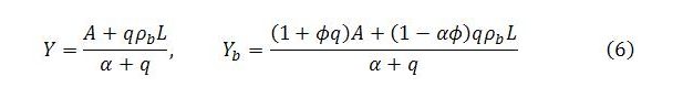
Corresponding expressions for the other endogenous variables are easily obtained. The steady state level of Yj is simply the expression for Gj multiplied by ϕ. The sectoral employment levels in a steady state will be Yb / ρb and Yj / wj.
An exogenous change in autonomous demand will cause multiplied changes in the steady state levels of the endogenous variables. These multipliers can be obtained by differentiating or taking the first difference of the relevant expression with respect to A:

Exogenous changes in total employment also have multiplier effects, which can be found by differentiating the various steady state expressions with respect to L. An individual decision to enter the labor force and take a job guarantee position will activate government expenditure on the program, with a multiplier effect on the economy. This is a notable aspect of the job guarantee in that an increase in supply-side potential automatically translates into higher demand. An earlier post considers a couple of effects along these lines. The present focus, however, will be on the expenditure multipliers.
The expressions in (5) and (6) can be arranged in various ways. The above arrangement is chosen for its succinctness and to provide a common denominator. As displayed, the expressions tell us the steady state levels of the endogenous variables given the values of the exogenous variables and parameters. But the form of presentation is not conducive to understanding the likely dynamics involved in moving from one steady state to another. This is a different question and the focus of subsequent sections of the post.
Before turning to that question, though, the meaning of q requires some explanation. A cursory glance at (5) and (6) reveals that the term appears in both the numerator and denominator of all the main expressions. It is a positive constant defined as
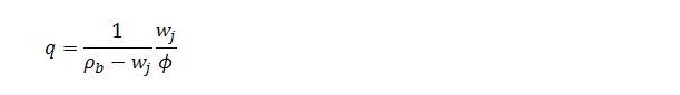
The margin ρb – wj is the additional income that is generated by having a unit of employment located in sector b rather than sector j. This margin is created because productivity in sector b is assumed to be higher than in sector j, where productivity is taken to equal the job guarantee wage on the basis that ρj = Yj / Lj = wj. The margin, then, is just the productivity differential.
Another way to think of the productivity differential is as the extra gap that is opened up between maximum possible income Ymax and income Y for every unit of employment that is located in sector j. In this interpretation, Ymax is taken to be the level of income that notionally could be generated if all employment were located in sector b. Looked at this way, the first term in q, which is the reciprocal of ρb – wj, can be understood as the marginal response of sector j employment to a unit widening of the income gap.
The second term in q, wj / ϕ, has already been encountered. As observed earlier, it represents job guarantee spending per unit of sector j employment.
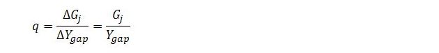
Combining these observations, q can be expressed in terms of changes:

So q measures the endogenous response of job guarantee spending to a widening of the income gap. Under present assumptions, it also expresses job guarantee spending as a fraction of the income gap:
2. A representation of dynamic adjustment
Here is a way to think about the dynamic adjustment process between two steady states that is analogous to the way the standard model’s dynamics are usually interpreted.
Beginning from a steady state, imagine a one-off exogenous change in demand that causes the economy to leave the steady state. Conceptually, we can suppose that this has an immediate impact on total income and sector b income but that the effects on job guarantee spending and household consumption are delayed.
Specifically, let ΔA denote the change in autonomous demand. At time t = 0, it is assumed that total income and sector b income change by the amount ΔA. At time t = 1, job guarantee spending and consumption respond to the events of time t = 0. This affects total income and sector b income in the same step. These changes in the level of income and its composition at time t = 1 then impact on job guarantee spending and consumption at time t = 2, with immediate impacts once again on income and its composition, and so on. The objective is to arrive at expressions describing the behavior of total income, sector b income, job guarantee spending and consumption (and, by implication, other endogenous variables) over time.
In general terms, the following process is envisaged.

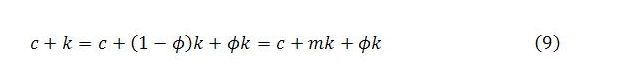
The abbreviations are to save space and make the algebra easier, with c = 1 – α being the net marginal propensity to consume. It is also convenient to let m = 1 – ϕ represent the fraction of job guarantee spending going to materials.
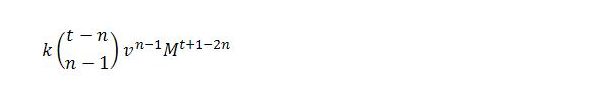
The negative fraction k is constant, given the values of the parameters. It measures the inverse response of job guarantee spending to variations in sector b income. A unit increase in sector b income results in 1/ρb units of employment switching from sector j to sector b and so causes a reduction in job guarantee employment of 1/ρb. Since government spends wj / ϕ per unit of sector j employment, the unit increase in sector b income causes job guarantee spending to change (negatively) by -(1/ρb)(wj / ϕ), or k. In terms of changes:

The immediate aim is to express changes in Y, Yb, Gj and C in terms of exogenous variables and parameters. This can be done by writing down appropriate equations for the first step, t = 0, and then using these initial expressions to write down appropriate equations for the second step, t = 1, and so on, until a clear pattern emerges. Excel or a similar spreadsheet package is extremely useful for checking that the equations actually work. Setting up a spreadsheet is much easier than deriving the equations. The simple recursive rules outlined in (8) are all that are required for that purpose.
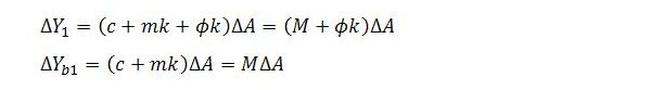
Applying the first of the rules in (8) for time t = 0 gives:

The endogenous expenditures will begin to respond in the next step, with further ramifications for income and its composition.
At time t = 1:

In the last line, use is made of the definition m = 1 – ϕ to express k – ϕk as mk.
Before continuing, it is helpful to note that
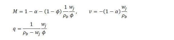
An effective strategy is to group c + mk terms together and let M = c + mk. When a c + k term appears, it can be split into an M term and a ϕk term in accordance with (9). The ϕk terms will get multiplied by c to generate ϕkc = v terms. So for convenience:
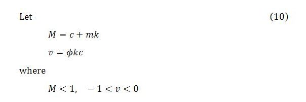
In economic meaning, M is the spending induced by an increment in sector b income, taking into account both induced consumption and countercyclical variation in job guarantee spending on materials. v is the (negative) change in sector j workers’ consumption caused by a one unit increase in Yb due to the latter’s effect on sector j employment and wages. This makes M + v the net marginal propensity to spend out of sector b income, taking into account both induced consumption and the inverse effects on consumption and materials expenditure of endogenous variation in job guarantee spending. So, in generating the equations, the net marginal propensity to spend out of sector b income will get decomposed into separate M and v terms. For given parameter values, M and v are constants.
Following this strategy, the expressions for ΔY1 and ΔYb1 can be restated as:
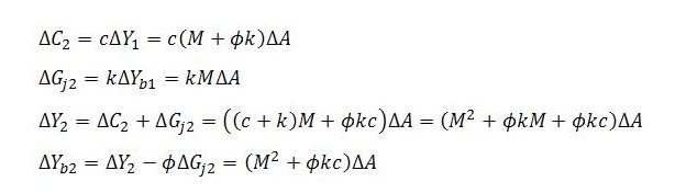
At time t = 2:
The overall pattern is not clear at this stage but emerges if we continue with the algebra for some more steps. Here, we will jump ahead a little and look at some of the expressions that emerge for early steps in the process. Energy can be conserved by focusing on the equations for Yb and Gj since these are pivotal and can be used to obtain corresponding expressions for the other variables.
To save a bit more space, changes in Yb and Gj will be divided by ΔA with the following notation adopted:

Continuing to work through the algebra gives the following changes in Yb per unit change in A for steps 0 to 9. The purpose here is to notice a pattern.

The pattern followed by the coefficients in (12) relates to Pascal’s triangle. The integers involved are figurate numbers that can be read off the diagonals of the triangle. The first terms in each row are preceded by a 1. The second terms, from t = 2 onward, are preceded by ascending natural numbers (1, 2, 3, …). The third terms, from t = 4 onward, are preceded by ascending triangular numbers (1, 3, 6, …). The fourth terms, from t = 6 onward, are preceded by ascending tetrahedral numbers (1, 4, 10, …). The fifth terms, from t = 8 onward, are preceded by ascending pentatope numbers (1, 5, 15, …). The pattern continues through the simplex numbers.
With the pattern now evident, it is possible to form an equation that describes the behavior of Yb. Focusing on the right-hand side of (12), the rows (or equations) can be numbered from t = 0 and the columns (or terms) from n = 0. The term in row t and column n will be
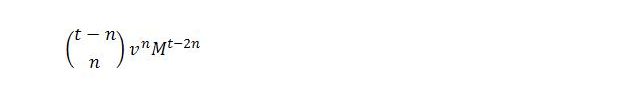
The first term in brackets is the binomial coefficient C(t – n, n). The change in Yb with respect to A at time t will equal the sum of the terms in row t:

Summing across all time steps gives the total multiplier impact on Yb of an exogenous change in demand:
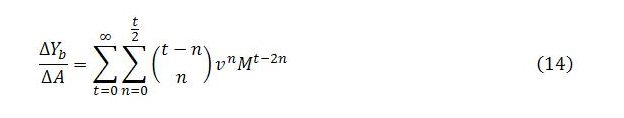
Together, these last two expressions give a description of Yb‘s behavior over time. Expression (13) enables us to calculate the change in Yb at a given time step, while (14) can be used to find the cumulative change over all or a subset of time steps.
The behavior of the other variables can be considered in the same way. Fortunately, it is only really necessary to retread the above steps for job guarantee spending. Once the behavior of Gj becomes clear, it will be easy to infer the behavior of the other variables from the combined behavior of Yb and Gj.
Working through time steps 1 to 9 for the changes in job guarantee spending gives:

The pattern is very similar to the behavior displayed by Yb except that it is lagged a step, with each term multiplied by k. In view of the lag, we can number the rows from t = 1. To avert possible confusion, the columns can also be numbered from n = 1.
The value of the term in row t and column n will be
The change in Gj with respect to A at time t is given by the sum of the terms in row t:

Summing across all time steps gives the full multiplier impact:

The corresponding expressions for Y can be obtained using the following relationships:

The expressions for C are most easily obtained from the resulting expressions for Y:

3. Conformity of the dynamics to steady state requirements
We now have expressions for the steady state levels of the endogenous variables. These were obtained in section 1. We also have expressions that describe the behavior of the endogenous variables at each step in time when they follow a simple set of recursive rules. These were obtained in section 2. But for the assumed dynamic behavior to be consistent with the underlying assumptions of the model, we need it to generate results that are the same as those implied by the steady state relationships. Specifically, the full multiplier impacts generated by the dynamic behavior should match the multipliers that are implicit in the steady state expressions and listed in (7). We need a way to compare the two sets of multipliers and verify that they are actually the same. For this purpose, it will be helpful to have formulas for the series sums developed in section 2 that are easy to compare with the multipliers in (7). Obtaining such formulas and showing that they are equivalent to the multipliers in (7) will verify that the assumed dynamics conform to the steady state requirements of the model.
A key to the exercise is to keep in mind that the sum of a geometric series with common coefficient a and factor r exists so long as r has an absolute value less than one.
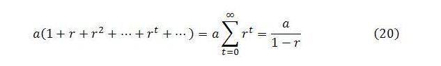
When the absolute value of r is less than one, the terms in the series approach zero as t becomes large, and the sum of the series converges on a finite point that can be calculated using the formula on the far right-hand side.
It will be possible to obtain summation formulas for the endogenous variables in the form of (20). As in section 2, most effort can go toward obtaining formulas for Yb and Gj because of the way they are connected with the other variables.
The full impact on Yb of an exogenous change in demand has been found to be:

Recall that this sum relates to a system of equations for ΔYbt / ΔA. The first equations in this system are shown in (12). In (14), terms in a given row of (12) are summed horizontally with the result added to the total of all previously summed rows. Each row pertains to a particular time step. This choice was useful for describing the behavior of Yb over time, which was our aim in section 2, but it is not so helpful for obtaining a formula for the sum of the series. For that purpose, it is more convenient to sum vertically down columns and add the column sums together.
Some of the equations for ybt = ΔYbt / ΔA are reproduced below for easy reference:

To sum vertically, we fix the value of n (which denotes a column) and sum over all values of t. The same can be done for all other values of n to obtain an expression for the total change in Yb.
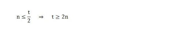
In summing the columns, care is needed in setting up the summation. In (14), the summation only applies to values of n that are less than or equal to t/2. This implies that we need to take the column sums for values of t greater than or equal to 2n:
The sum of column n will be
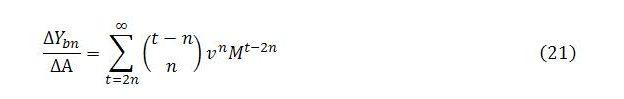
The limits of this summation can be shifted so as to start each column sum from t = 0:

As was noted earlier, the coefficients in (12) are figurate numbers. These numbers can be represented in terms of rising and falling factorials. To match our notation, let n represent the “type” of number in Pascal’s triangle, with n = 0 denoting ones, n = 1 denoting natural numbers, n = 2 denoting triangular numbers and so on. The t th number (t = 0, 1, 2, …) of type n will be given by the formula

Here, n bar is the n th rising factorial of t and n! is the factorial of n. By definition, zero factorial equals 1.
To give a couple of examples, the fourth triangular and seventh tetrahedral numbers are

This way of representing the numbers in Pascal’s triangle can be applied to the equations in (12). Column n in that system of equations contains numbers of type n. The t th nonzero entry in the column will be the t th number of type n.
Using this notation, (21′) can be written as
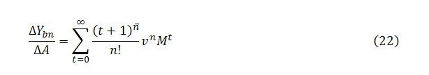
As has been noted, this is the sum of column n. We want to find a simple formula for this sum. A way to find the formula is to substitute successive values for n into (22) and look for a pattern. The strategy is as follows. Each time a value for n is substituted into (22), treat the resulting expression as a function of M. By integrating the function n times with respect to M, it will be possible to isolate a ΣMt term. The formula for the sum of a geometric series given in (20) can then be applied, with a = 1 and r = M, to replace ΣMt with 1/(1 – M). With this replacement made, the function can be differentiated n times with respect to M to eliminate any constants of integration and solve for f (M) = ΔYbn / ΔA.
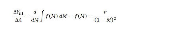
When n = 0, (22) becomes:

When n = 1,

Since n =1, we now integrate once with respect to M. The t + 1 term will cancel:

K1 is a constant of integration. Differentiating with respect to M and solving:
A pattern is emerging. We can go over some of the procedure one more time to check.
Letting n = 2,

Without actually performing the integrations it is clear that the first integration will eliminate the t + 1 term and the second integration will eliminate the t + 2 term. M will be raised to the power of t + 2. M2 can be taken outside the summation, leaving only ΣMt on the inside, which can be replaced with 1/(1 – M). This will give:
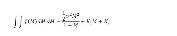
where K1 and K2 are constants of integration. Differentiating twice with respect to M gives:

The procedure gets more laborious as n is increased because of the need to integrate and differentiate n times, but the pattern is clear. All terms in the numerator other than vn cancel out after the n th differentiation and we are left with an expression in the form:
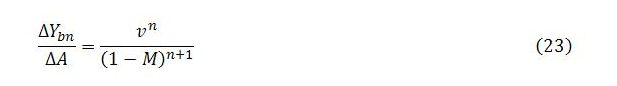
This expression gives the sum of column n in the set of equations abbreviated in (12).
The total multiplier impact on Yb is obtained by summing the totals of all the columns:
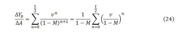
Conveniently, (24) is in the form of a geometric series, as shown in (20), with a = 1/(1 – M) and r = v/(1 – M). Plugging into the formula in (20) gives:

So long as the system converges to a steady state, this formula gives the full multiplier impact on Yb of a change in autonomous demand when behavior follows the simple recursive rules outlined in (8).
For Yb to converge, it is necessary that:

Keeping in mind that M + v is the net marginal propensity to spend out of sector b income, convergence will occur for appropriate values of the parameters.
Mathematically, divergence would occur if either M + v > 1 or M + v < -1. But neither of these cases is plausible. The first case is impossible so long as there is a positive marginal propensity to leak (α > 0) because M always takes a value less than one and v is defined to be negative. The second case would make no sense from a policy perspective. For M + v to be negative at all, let alone less than -1, a unit increase in sector b income would need to be accompanied by a withdrawal of job guarantee spending that more than offset the extra induced consumption. The main way it could happen mathematically would be for the fraction of job guarantee spending on wages (ϕ) to be unrealistically small. For example, for α = 1/2, ρb = 2 and wj = 1/2, divergence would occur for a value of ϕ less than 2/15. For ϕ of exactly 2/15, the system would oscillate from one time step to the next with sector b income showing no tendency either to rise or fall. Or with α = 1/5, ρb = 3 and wj = 1/2, the system would diverge for values of ϕ less than 5/63. These choices for ϕ would be inapplicable from the policy perspective. On economic considerations, the system will always converge.
We are now in a position to compare the multiplier impact generated by our assumed dynamic behavior, given in (25), with the multiplier for Yb that was derived from the steady state relationships and listed in (7). If the two multipliers happen to be the same, the assumed dynamics will not violate steady state requirements. Our conceptualization of the dynamics will be consistent with the underlying assumptions of the model.
The steady state relationships imply a multiplier for Yb that is shown in (7):

We need to compare our formula in (25) with (26). To do so, it is necessary to substitute in the actual expressions for M and v, since these terms are abbreviations chosen to conserve space. It is also necessary to recall the definition of q. For convenience, these are reproduced below:
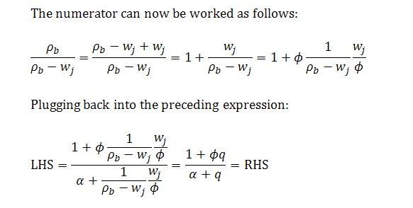
It needs to be shown that:
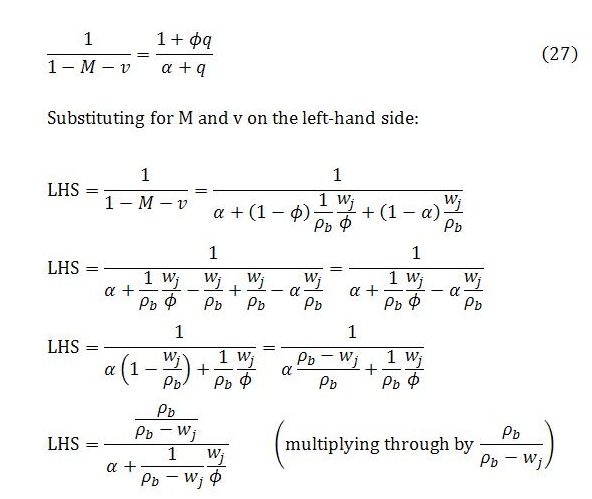
This verifies that the multiplier impact on Yb generated by the assumed dynamic process matches the multiplier impact implied by the corresponding steady state expression. In other words, the dynamics of sector b income conform to steady state requirements. For given values of the exogenous variables and parameters, the assumed system behavior will cause Yb to converge on its steady state level, as depicted in (6).
Convergence of other variables
The approach just taken for sector b income can also be applied in the case of job guarantee spending. By summing vertically down each column of the system of equations for gjt = ΔGjt / ΔA it is possible to arrive at a simple formula for the sum of a series. This formula will be equivalent to the multiplier derived for Gj on the basis of steady state relationships. Once equivalence is established for the multipliers of both Yb and Gj, it is straightforward to handle Y, C and, by implication, Yj and other endogenous variables because their expressions can all be obtained from those for Yb and Gj. Specifically,

It is unnecessary to go into the same detail for Gj as we did for Yb as the steps and algebra are almost identical. But there are a few points that might be unclear without some elaboration.
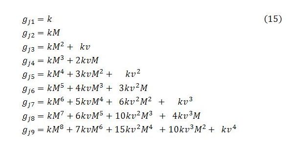
The gjt for t = 1 to t = 9 are reproduced below:
Before summing vertically, it is once again important to consider the limits of summation in the expression for the total change in Gj:

The summation only applies to values of n that are less than or equal to (t + 1)/2. So we need to take the column sums for values of t greater than or equal to 2n – 1:

The sum of column n will be

Left as it is, this would be inconvenient for integrating and differentiating n times. It helps to shift the limits of the summation so as to start each column sum from t = 0:

Replacing the binomial coefficients with equivalent expressions involving rising and falling factorials and treating ΔGjn / ΔA as a function of M gives us a convenient starting point:

From here there are no surprises. For each n, we integrate n times to get a ΣMt term by itself that can be replaced with 1/(1 – M). We then differentiate n times to eliminate the constants of integration and solve for f (M).
As might be guessed, the end result is a formula that is almost identical to the one for the total change in Yb except that the numerator is multiplied by k.
Similar expressions for the other variables can be obtained from those for Yb and Gj. The resulting formulas are all equivalent to the corresponding multipliers implied by the steady state expressions. The various multipliers resulting from the assumed dynamics are shown below.

4. Concluding remark
The focus has been on a model economy with a job guarantee. Adopting the income-expenditure model as a base, we identified characteristics of a steady state and described a dynamic process – analogous to the usual dynamic interpretation of the base model – that would tend to bring the system, when outside a steady state, back toward it.
Appendix
A fair bit of notation has been used. For easy reference, it is summarized below.