The model as outlined so far implies particular dynamics. These dynamics are driven by the quantity response of the broader economy (sector b) to mismatches in supply and demand. With the size of the labor force, level of total employment, within-sector productivity and the economy’s productive capacity all taken as exogenously given, the quantity response of sector b requires a change in the sector’s level of employment. The response of sector b induces an inverse response from the job-guarantee sector (sector j), which adjusts as required to maintain full employment at all times. The resulting variations in the composition of employment between higher-productivity sector b and lower-productivity sector j enable the adjustment of total output to total demand.

 
Preliminaries

Levels and rates. In what follows, the focus is on the levels of total output, total demand, sector b output and sector j output (denoted Y, Y_d, Y_b and Y_j, respectively) and their growth rates (g, g_d, g_b and g_j, respectively).

In continuous time, the instantaneous growth rate of a variable is its time derivative divided by its level. For example, the growth rate of total output is Y’/Y, where Y’ = dY/dt and t represents time. Or, for any variable x that can be considered a function of time, the instantaneous growth rate of x is x’/x, where x’ = dx/dt.

Definitions. Some of the results to be presented can be expressed more compactly by defining two ratios, q and k.

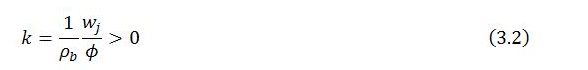
The first of these ratios, q, has already been introduced in part 2. It expresses job-guarantee spending as a fraction of the output gap,

Here, ρ_b is sector b productivity, w_j the job-guarantee wage (and sector j productivity) and ϕ the fraction of the government’s job-guarantee spending that goes to wages. At the moment, ρ_b, w_j and ϕ are all taken as given, making q a constant.

The second of the ratios is

This is the derivative of job-guarantee spending with respect to sector b output, ignoring sign. Under present assumptions, k is constant. A change in sector b output induces a proportional change in job-guarantee spending of dG_j = -kdY_b.

It follows from definitions (3.1) and (3.2) that

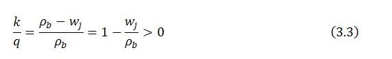
In words, k/q is the productivity differential expressed as a fraction of sector b productivity or, equivalently, one minus the quotient of the sectoral productivities.

 
Output levels

Sector b output. The dynamics of the model follow from the assumed response of the broader economy to excess demand or excess supply. In particular, it is supposed that sector b output changes in some positive proportion λ to excess demand:

If y = Y_d/Y is adopted as an alternative representation of excess demand, the response function can instead be written

Output of the broader economy expands (Y_b‘ > 0) when there is excess demand (y > 1) and contracts (Y_b‘ < 0) when there is excess supply (y < 1).

Sector j output. The job-guarantee sector reacts to the behavior of the broader economy. With sector j output evaluated as the wages paid to job-guarantee workers (Y_j = w_jL_j) and within-sector productivity taken as given, the change in sector j output is inversely proportional to the change in sector b output:

Substituting for Y_b‘ using (3.5),

Total output. The change in total output is simply the sum of the sectoral adjustments:

Illustration. Suppose the exogenous variables and parameters initially take the following values with the economy in a steady state:

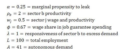
Given these values, k = 0.375 and q = 0.5.

In the initial steady state,

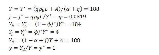
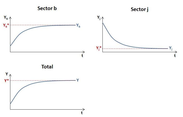
Imagine now that there is a unit increase in autonomous demand from its initial level of 41 to 42. This temporarily lifts y above one and causes total and sectoral activity levels to tend toward a new steady state with the following characteristics:

The adjustment of total and sectoral output levels to the new steady state is illustrated below. The graphs are not to scale.

 
Output growth rates

The growth rates of total output, sector b output and sector j output will be Y’/Y, Y_b‘/Y_b and Y_j‘/Y_j, respectively. Recalling from part 1 that Y_b = (1 – ϕj)Y and Y_j = ϕjY, these growth rates can be expressed in the following form:

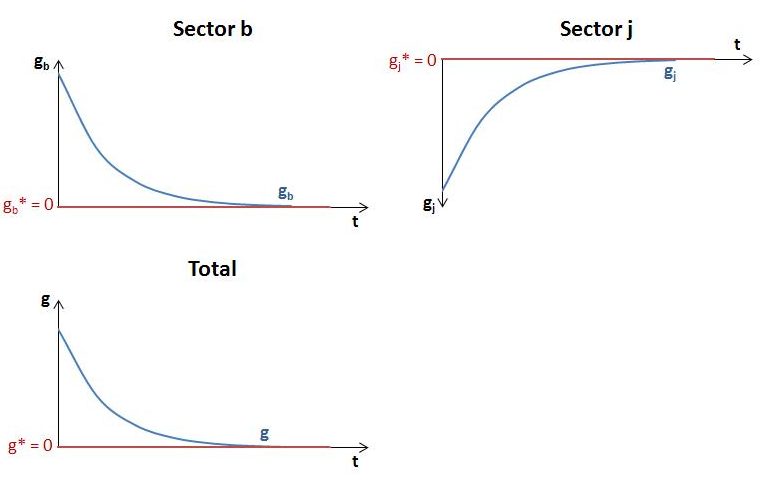
In a steady state, y = 1 and the growth rates are all zero. Excess demand or excess supply causes y to diverge from 1 and the various growth rates to differ from zero until the steady state is restored.

Illustration. Continuing with the same example, a unit increase in autonomous demand displaces the sectoral and economy-wide growth rates from the steady state until the adjustment process is complete.

 
Growth rate of total demand

Total demand is the sum of induced and autonomous elements:

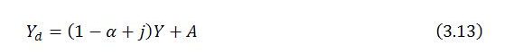
In this expression, α is the marginal propensity to leak to taxes, saving and imports, and j is the share of job-guarantee spending in total income. Recalling from part 2 that

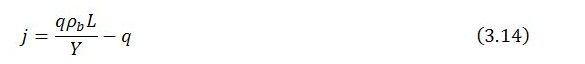
total demand can be written

Differentiating with respect to time (treating q, ρ_b, L and A as constants), dividing both sides by Y_d and multiplying the right-hand side by Y/Y gives

The growth rate of demand is zero in the steady state, which occurs when supply equals demand (y = 1). The growth rate of demand can also be zero despite the presence of excess demand or excess supply if the sum of α and q just so happens to equal one. This corresponds to the special case of a horizontal demand schedule in the Keynesian cross diagram mentioned in part 2. Other than in this special case, the growth rate of demand will deviate from zero whenever y diverges from one.

Illustration. For α + q < 1, a positive demand shock causes g_d to be positive until the adjustment process is complete. For α + q > 1, a positive demand shock causes g_d to be negative throughout the adjustment process. If α + q = 1, total demand is impervious to shocks.

In our ongoing example, α + q < 1. The adjustment of total output to total demand for this case is illustrated in the final diagram. The adjustment of total output is achieved through an expansion of sector b and contraction of sector j. This causes the share of job-guarantee spending in total income (j) to decline toward its new steady state value j*.