
In recent parts of the series, we have been considering the temporal single-system interpretation (TSSI) of Marx’s theory of value. We have considered how, in the TSSI, the values of constant capital and variable capital depend upon the prices that prevail when inputs and labor power enter production. In contrast, the values and prices of output are only determined once production is complete and the commodities are ready for sale on the market. This conception of value and price determination requires a more general formula for the MELT (or ‘monetary expression of labor time’). The basic meaning of the MELT remains the same. It is still the amount of monetary value attributable to an hour of socially necessary labor or, conversely, the amount of labor, represented in commodities, that a unit of the currency can command. But there is now a need to account not only for the rate at which living labor creates monetary value but also the rate at which monetary value is transferred from the means of production to final output. In the TSSI, the method for calculating the MELT needs to be modified under most circumstances.
The present purpose is to:
- Introduce the temporal MELT;
- Demonstrate, by applying the concept of the temporal MELT, that the TSSI upholds Marx’s view that surplus labor is the sole basis of real profit;
- Explain how the operation of the temporal MELT modifies the macro connections considered in parts 1 and 2 of the series.
The present post is largely focused on technical considerations. Although technical, and a little algebra heavy, the math involved is actually very simple. A numerical example is provided at the end to illustrate the use of the various formulas. A few straightforward derivations are relegated to an appendix.
Note. Discrete or continuous time. As with part 4 of the series, value and price determination will be considered here within a discrete period of time. It is possible to analyze the process in continuous time. This has been done, for example, by Freeman (1996). (See also Kliman 2001, p. 107). Formulating the TSSI in continuous time does not alter any of the important conclusions. For present purposes, nothing is lost by sticking with discrete time. As in part 4, it will be assumed that inputs and labor power enter production at time t and that output is ready for sale at time t+1. In other words, the period – considered to be period t – begins at time t and ends at time t+1.
Notation. To be consistent with part 4, time subscripts are applied as follows. Variables determined at time t have a t subscript. Examples are constant capital and variable capital expressed in monetary terms and the start-of-period temporal MELT. Variables determined at time t+1 have the subscript t+1. Examples are total price, the dollar value of surplus value and the end-of-period MELT. Variables that describe processes occurring over the entire period carry no time subscript. Strictly speaking, they should have the subscript t,t+1. To simplify the notation, these subscripts are omitted, but the variables should still be thought of as referring to what occurs over the whole period. Examples include living labor performed and surplus value expressed in labor time.
1. The MELT when prices and productivity are free to vary
Calculating the temporal MELT. In the first two parts of the series, the general price level and average productivity were assumed to be constant. This meant that the MELT could be expressed as m = Pρ, where P is the price level and ρ average productivity. Since P and ρ were assumed constant, the MELT was also constant.
In the present post, these assumptions are relaxed. Once the price level and productivity are free to vary, the simple relationship between m, P and ρ no longer holds in quite the same way. Even so, there is still a close connection between the variables as will be explained.
A more general expression for the MELT is:
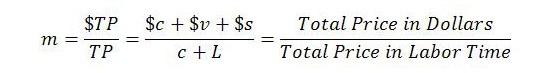
In the TSSI, it is also necessary to account for the sequential nature of value and price determination. In principle, working out total price in dollars is relatively straightforward once the period is over:
![]()
Calculating total price in labor-time terms is a bit more involved because the elements of constant capital are purchased at period t prices, whereas output is valued and priced at time t+1.
The monetary amount paid for constant capital needs to be converted into the equivalent magnitude of labor time. This is done by dividing $ct by the start-of-period MELT, mt. The start-of-period MELT is often referred to as the ‘input MELT’, because it applies to inputs. The two terms can be used interchangeably.
Output prices are determined later, at time t+1. Accordingly, total money price needs to be divided by the end-of-period MELT, or ‘output MELT’, mt+1. This converts total money price into the equivalent amount of labor time.

Variable capital does not present the same difficulty for value and price determination because it is replaced by an amount of living labor. As discussed earlier in the series, Marx argued that an hour of socially necessary labor always creates the same new value, in real terms. This is a very useful rule to keep in mind at the aggregate level. It means that no matter how productivity changes, a given level of employment L will always create the same new value. At the macro level, higher productivity simply means that the bar on what counts as socially necessary labor has risen. If we know the level of employment of the previous period, then the amount of new value added in the current period can be determined by comparing this period’s employment to that of the previous period.
We are now in a position to express total price in real, labor-time terms:
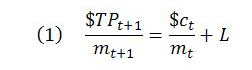
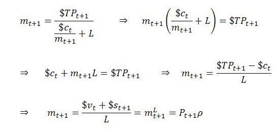
Rearranging (1) provides a formula for the temporal MELT, which was first presented by Ramos-Martinez (2004, p. 75) with somewhat different notation:
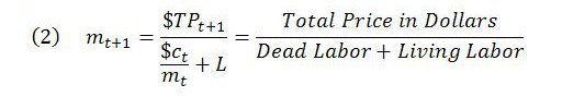
As (2) indicates, the output MELT, mt+1, depends partly on the input MELT, mt. In principle, the input MELT can be known at time t. It is a given datum for the current period. This underscores the sequential nature of value and price determination in the TSSI. The prices of inputs (which affect the value of constant capital) and the input MELT are results of history and now serve as data for the new period.
In the special case of a constant MELT, the formula for the temporal MELT reduces (apart from the temporal aspect) to the formula we used in part 1 of the series:
This can be seen by setting mt = mt+1 in (2) and rearranging, noting that $TPt+1 is equal to the sum $ct + $vt + $st+1. The simple algebra is left for appendix A1.
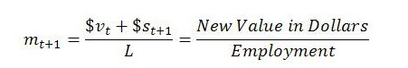
The monetary expression of living labor. For present purposes, it will be instructive to define the ‘monetary expression of living labor’ (MELL) as the ratio of new value in dollars to total employment:
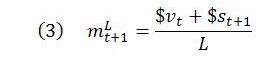
Referring back to the previous expression makes clear that when the MELT remains constant from one period to the next, the temporal MELT equals the MELL, as defined in (3). In this special case, the MELT depends only on the ratio of new value added to living labor performed over the period.
In the context of simultaneous valuation, the MELL in fact coincides with the definition of the MELT. It is only in the temporal framework of the TSSI that a distinction emerges. Perhaps for this reason, there has not been much explicit discussion of the MELL by that name, as far as I am aware. Even so, the concept never seems to be too far from the surface. The term is mentioned explicitly by Itoh (2005, p. 180). Similarly, Ramos-Martinez (2004, p. 72) refers to “the MELT corresponding to living labour”.
As with the simultaneist MELT, the MELL can be expressed as:
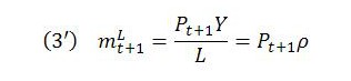
where Y is real income or real output. In the presence of fixed capital, Y needs to be understood net of depreciation. This is because, in Marx’s theory, depreciation is included in constant capital rather than gross income. So the MELL, as well as being defined as new value in dollars divided by employment, can also be thought of as the ratio between net domestic product (NDP) and employment. The MELL is also equal to the price level multiplied by average productivity. When it is assumed for simplicity that there is no fixed capital, as was done in parts 1 and 2 of the series, the MELL becomes the ratio of GDP to employment.
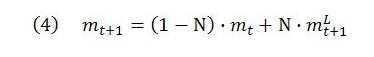
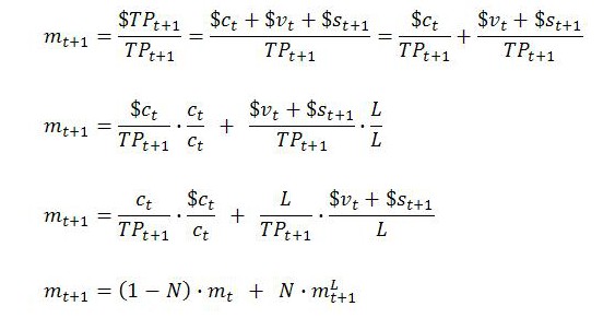
One benefit of defining the MELL is that it enables us to express the temporal MELT at time t+1 as a weighted average of the start-of-period MELT and the end-of-period MELL. (See appendix A2 for the details.) Specifically, it can be shown that:
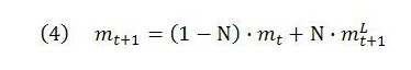
Here, Ν is the ratio of living labor to total price expressed in labor time. This makes 1 – Ν the ratio of dead labor to total price in labor time.

For Marx, total price equals total value. Therefore, the weights reflect the proportions of total value that are created by living labor (Ν) or transferred from dead labor (1 – Ν). They can be thought of in another way by noting that total price equals total (both living and dead) labor. From this perspective, the weights reflect the ratios of living and dead labor to the total labor either performed or transferred to final output over the period.
The concept of the MELL can also help to illustrate the way in which the temporal MELT reflects historical movements in prices and productivity. Conceptually, the temporal MELT can be likened to a weighted average of present and past MELLs; that is, as a series of present and past products of P and ρ. The further in time we go back, the more accurate this representation becomes.
The reason for this is that the MELT of a particular period can be expressed as a weighted average of past and present MELLs plus the start-of-period MELT taken from the earliest period considered, which will have a near-zero weight. The way to show this is presented in appendix A3. But the basic approach is to apply the formula for the temporal MELT in (4) to successive periods.
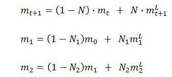
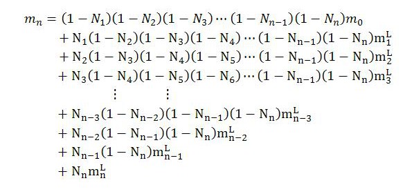
Suppose we are considering n periods in which period 0 is the earliest and period n the most recent. Using (4), first the formula for period 1 can be written down. The output MELT will be m1. The input MELT will be m0, the output MELT of period 0. Then the formula for m2 can be written down. Since m1 becomes the input MELT for period 2, the expression for m1 can be substituted into the expression for m2. This will express m2 in terms of the MELLs of periods 1 and 2 as well as the output MELT of period 0. The procedure can be repeated until the MELT for the most recent period, mn, is obtained. Time subscripts need to be attached to the Ν-terms (ratios of living labor to total labor) of each period. The effect of this procedure is to replace the start-of-period MELT in the most recent n periods with MELLs.
In this way, the temporal MELT for period n can be expressed in terms of n past and present MELLs along with the output MELT of period 0:

In (5), the output MELT of period 0 is multiplied by a product of n terms of the form (1 – Ν). Since Ν always takes a value between 0 and 1, this product approaches zero as n becomes large.
The MELL of each period is multiplied by its weight (one of the ϖt, where t = 1,…,n) and the resulting products summed. The weights are as follows:

We know that the MELL of each period is equal to the price level multiplied by productivity. With this in mind, (5) depicts the temporal MELT of the current period as the product of historical movements in productivity and prices. Recent history has the biggest impact, because the weights applying to the MELLs of the more distant past comprise products of many fractions and so are approximately zero.
In the calculation formula for the temporal MELT provided in (2), the sum effect of the entire history of price and productivity movements is conveniently captured in mt, the start-of-period MELT.
Infinite regress? It might be wondered whether the temporal MELT involves a problem of infinite regress. This period’s MELT takes the previous period’s MELT as a datum. So, how could the first ever temporal MELT be calculated?
Consider the formula again:

Logically, the resolution would appear to be a zero value for constant capital in the very first period of commodity production. If $ct = 0, the MELT depends only on the ratio of new value added in dollars to new value added in labor time (the current-period MELL). In that case, there would be no need for a start-of-period MELT.
Yet, we know that there will always be some raw materials used in production. (Even a nude mime artist will require physical space in which to perform.) So, what could explain a zero value for constant capital?
It is difficult to conjecture here, with the economic history of ancient civilizations hazy. But a possible answer might be that if we went back to the dawn of commodity production, which could have been simple commodity production, it seems likely that the first raw materials used to produce the commodities were not actually purchased but rather acquired with land or other private property that was granted by government or the community, or was otherwise claimed, seized or stolen. If no money was advanced for the raw materials used in the production of the very first commodity, then constant capital (as understood in single-system interpretations of Marx) would have been zero. The initial advance of capital would have been solely in the form of variable capital; that is, wages or some other form of sustenance for workers. If so, the formula for the temporal MELT would have been operable without the existence of a prior MELT.
It does actually seem difficult to conceive of the very first commodity being produced without the raw materials having been freely acquired. If there had been monetary payment for the raw materials, then the commodity requiring those raw materials as inputs would not have been the first commodity. At the very least, the raw materials would have been sold as commodities first. We would be looking at the wrong candidate for the status of first ever commodity.
Inflation in terms of the MELT. Over time, there is a tendency for the MELT to rise. According to Marx, an hour of labor, on average, always creates the same value in real terms. But its monetary equivalent typically rises over time. The rate of inflation, in terms of the MELT, is defined as:

A dot above a symbol (in these expressions, above m) indicates that the term refers to the rate of change of a variable. Here, it is the rate of change in m, or the inflation rate of the MELT. To deflate a monetary sum at time t+1 to period t prices, we divide it by one plus the rate of inflation. To inflate a monetary sum at time t to period t+1 prices, we multiply it by one plus the rate of inflation.
We have seen that the movement of the MELT over time largely reflects present and past changes in the MELL or, equivalently, present and past changes in prices and productivity. It is also possible to flip this around to consider the behavior of inflation in the general price level:

In the final part of this expression, λL is real (labor-time) net value added per unit of output. It is that part of unit value that is created by living labor rather than transferred from dead labor. This last part of the expression implies that the rate of inflation in prices will be approximately equal to the sum of the growth rates of the MELL and real unit net values:
![]()
This follows because of the mathematical rule that if x = yz, then x grows at the combined growth rate of y and z. The behavior of real unit values is strongly linked to productivity. Improvements in productivity have the effect of reducing the real values of commodities over time. For price inflation to occur, the MELL needs to rise more rapidly than real unit values fall.
It would also be possible to state an equally simple relationship between the price level, productivity and the MELT if we were prepared to adopt a broader than normal definition of productivity. (Kliman 2007, p. 109, note 2 may be alluding to something more or less along these lines.) If so, we could define a ‘total price level’ PT applying to all turnover T (including the elements of constant capital) rather than just net output Y, and also define ‘total productivity’ ρT to express the rate at which ‘total labor’ LT is both performed by living labor and transferred from dead labor to final output, considered in relation to total turnover.
In that case,
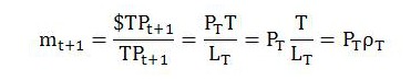
Rearranging the above expression gives:

This suggests that all prices, including of intermediate goods, will rise at a rate reflecting the combined growth rate of the MELT and real unit values. This relationship – or something similar – appears to be described by Kliman (2007, pp. 129, 137, note 11).
2. Surplus labor as the sole creator of profit in real terms
The algebra in this section closely follows Kliman (2001, pp. 106-109; 2007, pp. 185-187).
Total profit in nominal terms can be calculated as:

In nominal terms, there could be profit simply because of inflation. The relevant profit measure for Marx’s theory must therefore be profit adjusted for inflation. In the TSSI, the appropriate measure of inflation is taken to be the rate of inflation of the MELT, as defined in (6). Real profit πR is calculated by deflating the dollar value of total price to period t prices. This requires dividing the total money price by one plus the rate of inflation. Or, by (6′), we can multiply total money price by mt/mt+1.
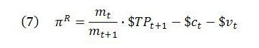
At this point it is convenient to multiply by mt each term in (1) – our earlier expression for total price expressed in labor-time terms – and then rearrange the resulting expression:

The first two terms on the right-hand side of (7) can now be replaced with mtL, noting also that $vt = mtvt.
![]()
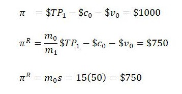
This confirms that in the TSSI, as for Marx, real profit equals the monetary equivalent of the surplus labor performed over the period.
Real profit will be positive whenever surplus labor is performed, provided the start-of-period (input) MELT is positive. Consider (2) again:

Since total money price and living labor are positive magnitudes and constant capital is nonnegative, the only way for a negative output MELT to occur would be for the input MELT to be negative. In other words, the output MELT will be positive provided the input MELT is positive. If the input MELT is positive, then the output MELT can never turn negative from that point onward. A positive input MELT in one period guarantees a positive output MELT for the current period, and this positive output MELT then becomes the input MELT for the next period.
There was initially some questioning in the literature of whether the input MELT could be assumed positive. The debate is discussed briefly in Kliman (2007, p. 187). Kliman and Freeman (2006) argued that a positive input MELT must always be the case. In support of their argument, they point out that an alternative way of defining the MELT is as the amount of labor a unit of the currency commands. For example, if the MELT is $20/hour, this means not only that one hour of socially necessary labor equals $20 of value but, conversely, that $1 commands (or can purchase) one-twentieth of an hour of socially necessary labor represented in commodities. They argue that since a unit of the currency must always have commanded a positive amount of labor, the MELT must always have been positive. Therefore, all subsequent MELTs must also have been positive.
Notice that the less labor a unit of currency commands, the higher (and so more positive) the value of the MELT becomes. So, establishing a positive MELT is not a high hurdle to jump. For starters, a unit of the currency could hardly command a negative amount of labor. The only possible hiccup remaining is that a unit of the currency might conceivably command zero labor.
My own view is that MMT’s notion of currency value z helps to confirm the TSSI position on this point. This is so if we are talking about the first MELT under capitalism. It might also be true under simple commodity production, but the relevant history is unknown. Capitalism depends critically upon a functioning state. The state, as enforcer of private property rights, is always in a position to ensure that a unit of the currency can command a positive amount of labor power (as distinct from labor). It guarantees this through enforcement of taxes. In fact, state enforcement of private property itself is likely to require the prior imposition of a tax obligation. Since most – and, if the state so desired, all – citizens of working age will either need to sell labor power in exchange for a wage, rely on somebody who does or endeavor to employ others to generate revenue in the currency in which taxes are owed, a unit of currency will always command a positive amount of labor power.
Now, if the state can always ensure that a unit of the currency will command a positive amount of labor power, then employment L will also be positive. That means there will be a positive amount of living labor performed. Recall that, for Marx, an hour of average labor always creates the same new value in real terms, irrespective of variations in productivity (Marx 1990, p. 137). This means that the labor performed will, on average, be value creating, and a unit of the currency, when used to purchase commodities, will command a positive amount of labor.
Actually, the value of the currency, defined in the MMT way, would seem to place a floor under plausible, persistent values of the MELT that will be well above zero. Not only will the MELT always be positive under capitalist commodity production, but it will be greater than 1/z unless profit is negative. For example, if all labor is simple and the wage rate is $10/hour, capitalists will not persist in initiating production that returns to them less than $10/hour of value. In other words, the value of the currency (its reciprocal) defines the minimum value of the MELT before capitalists will respond by ceasing commodity production. Conversely, and equivalently, the value of the currency defines the maximum amount of labor, represented in the commodities capitalists own, that a unit of currency can command (for customers) before capitalists will cease production. To the extent that a unit of currency commands less labor than labor power, capitalists pocket the difference as profit (apart from net taxes) and the MELT exceeds 1/z.
3. Modifications of some key macro connections
In the opening two parts of the series, under special assumptions, the following macro connections were emphasized:

To hold, these relationships required the price level and productivity to remain constant. Also relevant in the case of (9) is that all labor has been assumed simple and paid the same wage. If this assumption is relaxed, then either the value of the currency needs to be defined in terms of average labor and the average wage or the MELT and aggregate markup need to be expressed in terms of simple labor.
Rather than get into these complications now, it will continue to be assumed in this section that all labor is simple and receives the same wage. This means that simple labor is the same as average labor and the minimum wage equals the average wage. The complications will be considered later in the series, and do not appear to be especially problematic. The simplifying assumption does not change anything of significance for the current discussion.
The price level and productivity. Once prices and productivity are free to vary, the relationship in (8) becomes slightly more complicated. Recall:
Since it is the MELL that now equals the product of the price level and productivity, (4) can be written:
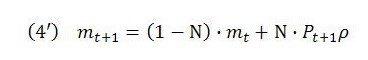
So, there is still a close relationship between the output MELT, the price level and productivity. Since the price level multiplied by productivity also equals new value added divided by employment, this ratio also remains closely connected to the MELT.
Below is an alternative way of expressing the temporal MELT in terms of new value added (see Kliman 2001, p. 108). In the expression, new value added is adjusted for inflation by inflating the monetary value of constant capital relative to total money price.

This is not a calculation formula. The output MELT enters both the left and right-hand sides. The expression can be rearranged to obtain:

The simple algebra required to obtain this expression is presented in appendix A4. The expression says that the end-of-period MELT is equal to the MELL (or price level multiplied by productivity) minus a correction for inflation that has occurred since time t when inputs were purchased.
The markup and value of the currency. Regarding (9), it was seen in part 2 of the series that the markup can be expressed in value terms either as ($v+$s)/$v or L/v. There was no difference between the markup in real terms or nominal terms because of our assumption that the MELT was constant.
Now that prices and productivity are allowed to change, it is necessary to distinguish between the nominal markup and the real markup. The definition of currency value, in contrast, is unaffected by the relaxation of assumptions.
The value of the currency, the markup in nominal terms and the markup in real terms kR can be expressed as:
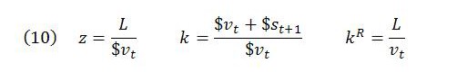
It follows from (10) that:
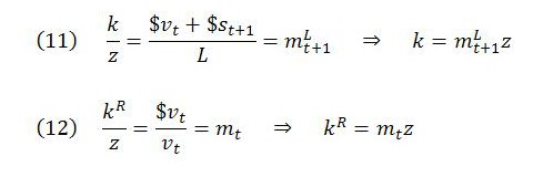
Both the nominal and real markups are closely connected to the value of the currency. In the nominal case, this connection operates through the MELL. In the case of the real markup, the connection operates through the start-of-period MELT.
It is also easy to express the real markup in terms of the nominal markup and vice versa. From (11) and (12):

The nominal markup is deflated using the input MELT and the MELL, rather than the output MELT, because the markup relates only to new value added.
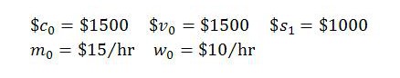
Numerical example. Suppose that the monetary outlays for constant and variable capital, valued at the prices prevailing at time t=0, are each $1500 and that the monetary amount of surplus value at time t=1 is $1000. Assume that the start-of-period MELT is $15/hour and the wage rate is $10/hour.
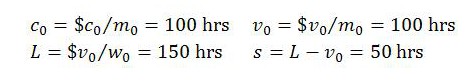
We therefore have:
This implies that:
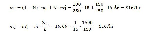
We are now in a position to calculate the MELT, MELL and rate of inflation in labor-time terms:

We can test our alternative expressions for the MELT:
We can calculate the markup, in real and nominal terms, as well as the value of the currency, and replicate the key macro connections:

The real markup is also equal to one plus the rate of surplus value (kR = 1 + s/v).
Finally, here are the calculations for profit in nominal and real terms:
APPENDIX
A1. When the MELT remains unchanged from one period to the next, it equals Pρ or, equivalently, the MELL. To show this, substitute mt+1 for mt in (2).
A2. It is possible to express the end-of-period MELT as a weighted average of the start-of-period MELT and the MELL.
A3. The MELT of period n can be expressed as a weighted average of the n present and past MELLs and the MELT of period 0. Working with the formula for the MELT just established above in section A2, start at period 1 and move forward in time, substituting the expression for an earlier MELT into the formula for the subsequent MELT. A pattern soon emerges.
The earlier expression for m1 can now be substituted into the expression for m2, and so on for later periods, until the pattern emerges.

Reordering terms:
A4. To express the output MELT in terms of new value added in the more realistic case in which the MELT varies from period to period, rearrange (2). The MELT can also be expressed in terms of the MELL.

References
Freeman, A. (2004), ‘Price, Value and Profit – A Continuous, General, Treatment’, in A. Freeman and G. Carchedi (eds.), Marx and Non-Equilibrium Economics, Cheltenham: Edward Elgar, pp. 225-279.
Itoh, M. (2005), ‘The New Interpretation and the Value of Money’, in F. Moseley (ed.), Marx’s Theory of Money: Modern Appraisals, New York: Palgrave MacMillan, pp. 177-191.
Kliman, A. (2001), ‘Simultaneous Valuation vs. the Exploitation Theory of Profit’, Capital & Class, Vol. 73, Spring, pp. 97-112.
Kliman, A. (2007), Reclaiming Marx’s “Capital”: A Refutation of the Myth of Inconsistency, Lanham: Lexington.
Kliman, A. and Freeman, A. (2006), ‘Replicating Marx: A Reply to Mohun’, Capital & Class, Vol. 88, Spring, pp. 117-126.
Marx, K. (1990), Capital, Vol. 1, London: Penguin.
Ramos-Martinez, A. (2004), ‘Labour, Money, Labour-Saving Innovation and the Falling Rate of Profit’, in A. Freeman, A. Kliman and J. Wells (eds.), The New Value Controversy and the Foundations of Economics, Cheltenham: Edward Elgar, pp. 67-84.
