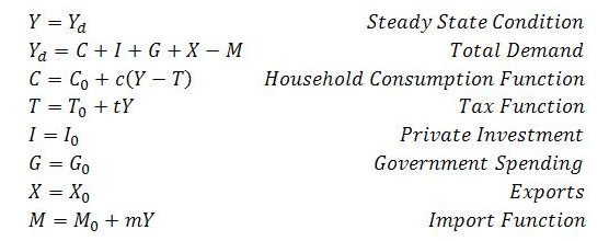
The following is mostly intended as background for a possible post (or posts) on quantity effects of a job guarantee in which the standard income-expenditure model is taken as a base. It is desirable to work from as simple a starting point as possible as the exercise can complicate pretty quickly. To minimize unnecessary complications, the base model will be presented in highly abbreviated form. This will not cause anything important to be lost because it is always possible to switch back to the more detailed version of the model when desired. The abbreviation has already appeared here and there in earlier posts, but to avert possible confusion it seems advisable to spell out exactly how it corresponds to the more familiar version of the model.
The standard model can be summarized in the following set of equations:
For the system to be in a steady state, output and income (both denoted Y) must equal demand Yd. Demand is defined as the sum of planned expenditures. These expenditures include household consumption C, private investment I, government expenditure G and net exports (exports X minus imports M). The other expressions are behavioral equations. In the simplest versions of the model, private investment, government spending and exports are all considered exogenous (denoted with a 0 subscript). Private consumption, taxes T and imports are endogenous. They are largely induced by income, though with autonomous components (C0, T0 and M0). The marginal propensities to consume, tax and import (c, t and m, respectively) are all assumed to be constants that take values between zero and one.
Through a series of substitutions the system can be solved for Y to obtain the steady state level of income:
The numerator of this expression is net planned autonomous expenditure, or ‘autonomous demand’. The denominator is the ‘marginal propensity to leak’. It is the fraction of an increment in income that drains to taxes, saving and imports. The model therefore depicts steady state income as a multiple of autonomous demand, where the ‘expenditure multiplier’ is the reciprocal of the marginal propensity to leak.
To condense the model, let A represent autonomous demand and α the marginal propensity to leak. The model can then be depicted more succinctly as
Demand, in (2), is the sum of induced consumption net of endogenous imports, represented by (1 – α)Y, and autonomous demand.
Substituting the expression for demand into steady state condition (1) and solving for Y gives:
As before, steady state income depends on the level of autonomous demand (now denoted A) and the marginal propensity to leak α. The multiplier, found by differentiating (3) with respect to A, is 1/α.
The model can be used to consider how a change in either the exogenous variable A or the parameter α will affect the steady state level of Y. If autonomous demand changes by the amount ΔA, the steady state level of income will change by ΔY = (1/α)ΔA.
As it stands, the model says nothing about how the system might get from one steady state to another. There are many conceivable ways this could occur. The one that is usually taken to make most sense goes along the following lines. An exogenous change in demand of ΔA will be the result of either an ‘injection’ (from one or more of government spending, private investment and/or exports) or autonomous household consumption, or some combination of the two. The extra exogenous spending will be received as income. This will induce additional household consumption on domestic output, as well as result in leakage or ‘withdrawal’ from the circular flow of income to taxes, saving and imports. In this way, a given increase in exogenous spending will initiate a multiplier process in which the newly created income induces consumption which, in turn, creates still more income, again inducing consumption, and so on. But the multiplier process associated with a particular act of autonomous spending eventually runs out of steam because withdrawals to taxes, saving and imports occur on each round of the process. Given the new value of autonomous demand and the marginal propensity to leak, there will be a stable (steady state) level of activity to which income converges.
The process just described suggests a power series. The idea is implicit in the expression for the multiplier. Since α is always between zero and one, 1/α can be interpreted as the sum of a convergent series. The sum of the series will be
The change in income caused by a change in autonomous demand can now be found by multiplying through by ΔA:
So, in the economic process envisaged, a change in autonomous demand of ΔA occurring at time t = 0 will be received as income. At time t = 1, a fraction 1 – α of this new income will go to consumption and be received as new income of (1 – α)ΔA. At time t = 2, a fraction 1 – α of this new income will go to consumption and create still further new income of (1 – α)2ΔA. And so on.
The basic logic of the model will remain the same when a job guarantee is included. But interaction between the broader economy and job guarantee program – which entails endogenous, countercyclical spending – modifies the steady state relationships and can especially complicate plausible representations of the system’s behavior when outside of a steady state.


