Under a job guarantee, there would be a standing job offer at a living wage for anyone who wanted such a position. Anyone without employment in the broader economy, or unhappy with their present employment, could opt for a position in the job-guarantee program. Similarly, individuals with less hours of employment than desired could top up their hours by working part-time in the job-guarantee program. In principle, the program might be locally or centrally administered. But, irrespective of administrative details, it will be assumed that a currency-issuing government funds the program.
One interesting aspect of a job guarantee, from an analytical perspective, is that it introduces an endogenous element to government spending. The government’s spending on the program will adjust automatically to variations in the number of people who accept the standing offer of a job. These variations will reflect employment fluctuations in the broader economy. Government spending will respond directly to employment fluctuations, and only indirectly to variations in income.
Given the level of autonomous expenditure (including the exogenous component of government spending) and the size of the expenditure multiplier, the overall level of government spending will depend on the rate of take-up of job-guarantee positions. Any endogenous change in government spending, linked to variations in job-guarantee activity, will have a multiplier effect in the broader economy that will then react back on the rate of migration between the two sectors as some workers respond to changing employment conditions in the broader economy. But this, too, by causing a change in the endogenous component of government spending and the accompanying multiplier effects, will create further feedback. The feedback effects between the job-guarantee sector and the broader economy will go back and forth, but their impacts will get smaller with each round of effects. This means that, in principle, it is possible to find a level to which government spending would converge, given the values of various parameters and exogenous variables. This is the present focus.
A simple model of output and employment determination under a job guarantee
To keep things relatively simple, consider a closed economy. (Extension to an open economy is straightforward, but adds nothing of interest to the point being considered.)
In an economy with a job guarantee, there is always full employment in the sense that anyone prepared to accept a job at a living wage has a job. Since average productivity in the job-guarantee sector may differ from average productivity in the broader economy, the level of output associated with full employment (Y = YF) will vary depending on the fraction of total employment that takes place in the job-guarantee sector. Under a job guarantee:
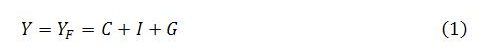
We can assume that private consumption includes autonomous and induced components, taxes are a constant proportion of income, and private investment is exogenous:
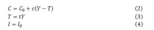
Substituting (2)-(4) into (1) and solving for full-employment income gives:

This looks familiar except that G represents total government spending, which is partly endogenous and the main focus of our attention. For convenience, we can define private autonomous expenditure as A’ = C0 + I0 and the marginal propensity to leak from the circular flow of income to taxes and saving as α = 1 – c + ct:

Let Yb and Yg be the levels of output produced in the broader economy and job-guarantee sector, respectively. The economy’s total output (Y) will be the sum of output produced in the broader economy and the job-guarantee sector: Y = Yb + Yg.
The output produced by the job-guarantee sector (Yg) can be measured as the amount that government spends on the program’s wages. It can be assumed that the cost of procuring material inputs involves government purchases of output produced in the broader economy. These ‘intermediate goods’ will not count towards production of the job-guarantee sector. Of the government spending on the job guarantee (Gg), only wages will contribute to the measure of the sector’s output. If ϕ is the proportion of job-guarantee costs associated with wages, then job-guarantee output is ϕGg. Accordingly, the economy’s total output can be expressed as Y = Yb + ϕGg. Rearranging gives an expression for output of the broader economy, Yb = Y – ϕGg. Or, using (5′):
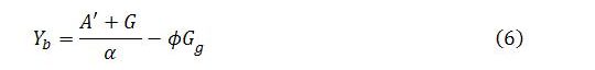
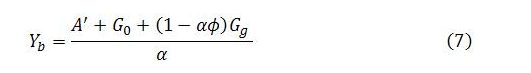
Total government spending (G) is equal to the sum of autonomous government spending (G0) and endogenous job-guarantee spending (Gg). That is, G = G0 + Gg. Substituting this expression for G into (6) and reworking yields:

The level of output in the broader economy is closely connected to the sector’s level of employment (Lb). Since average productivity in the broader economy is ρb = Yb/Lb, it follows directly that Lb = Yb/ρb. So employment in the broader economy can be calculated by dividing both sides of (7) by the sector’s average productivity:

The main task is to find an expression for endogenous government spending Gg. This will also suggest an expression for total government spending G.
The amount the government spends on the job guarantee (Gg) will be equal to the level of employment within the program multiplied by the cost of running the program per unit of employment. The first factor, the level of employment in the job-guarantee program (Lg), is equal to LF – Lb. To characterize the second factor, the cost of the program per unit of employment, let wL represent the living wage paid to job-guarantee workers per unit of employment and recall that ϕ is the share of wages in the total cost of the program. This makes the fraction wL/ϕ the cost of the program per unit of employment.
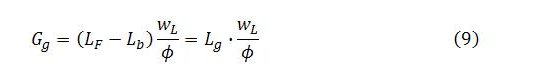
The level of employment associated with full employment (LF) is exogenous, determined by workers themselves. The living wage (wL) and wage share in costs (ϕ) are also exogenous. The living wage is set by government. The wage share in costs depends on the living wage, the prices government agrees to pay for equipment and materials, and the production techniques employed.
Unlike other terms on the right-hand side of (9), employment in the broader economy (Lb) is determined endogenously in accordance with (8). This expression for Lb can now be substituted into (9):
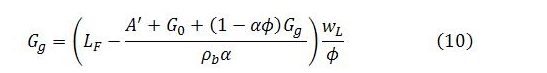
The term Gg appears on both sides of (10). The expression can be solved for Gg by expanding the right-hand side, grouping all terms involving Gg on the left-hand side, factorizing those terms and dividing both sides by the resulting factor. This yields:

Total government spending is the sum of the autonomous and endogenous components of government spending: G = G0 + Gg. Substituting the right-hand side of (11) into this expression for G and solving gives:

Expression (12) can be used to calculate the level to which government spending converges given particular choices for autonomous spending (G0 and A’), the level of employment corresponding to full employment (LF), the marginal propensity to leak (α), productivity in the broader economy (ρb), the living wage (wL) and the wage share in job-guarantee costs (ϕ). Alternatively, expression (11) can be used to calculate the level to which government spending on the job guarantee converges, given the values of the same parameters and exogenous variables, with the level of Gg then added to G0, the amount of autonomous government expenditure.
The direct social determination of productivity in the job-guarantee sector
Productivity always has a social determination. In the case of private-sector production, this point is often lost, because the social determination is played out through social institutions such as the market that many people come to see as natural. However, market outcomes depend, among other things, on distribution, which strongly influences the composition of demand and hence the composition of output and employment as well as the types of production techniques that are developed.
In the case of public-sector production, productivity can be conceived in a way that makes its social determination much more direct. Specifically, if public-sector output (Yu) is measured as the wages paid to public-sector workers (Wu), then it follows that productivity of the sector (ρu) can be viewed simply as the average wage per unit of public-sector employment (Lu):
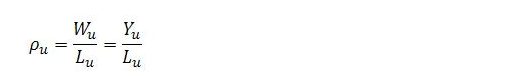
This determination of productivity is, in principle, democratic, based on “one person, one vote”, as opposed to the market, which is democratic only in a much more limited degree, characterized as “one dollar, one vote”.
For instance, the market would deem the provision of health care to the poor as of zero productivity unless somebody with private means happened to be willing to pay for it, since the poor lack the means to pay out of their own private income. Yet, if the poor were gifted income or received a transfer payment sufficient to pay for health care, the market would suddenly deem the same activity as having positive productivity.
A market assessment of productivity can only be valid to the extent that the distribution of income and wealth is legitimate. More generally, a market assessment of productivity is only valid to the extent society as a whole deems it to be valid. Even leaving aside distribution, markets often perform poorly due to externalities, public goods or coordination failures. If, for whatever reason, the social consensus is to reject the market’s verdict on the productivity of an activity, then it is the market’s verdict that is to be rejected. Under a job guarantee, as in public-sector activity more broadly, society would take a more direct approach to the assessment of productivity.
It has been noted that only part of the government’s spending on the job guarantee would result in output for the sector. The government’s spending on the program is represented by (9), which is reproduced below for convenience:

The output of the job-guarantee sector (Yg) can be measured as the wages paid in the sector (LgwL). Inspection of (9) reveals that job-guarantee output can be obtained by multiplying both sides of the expression by ϕ:
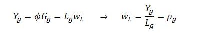
Defining productivity in the job-guarantee sector as ρg = Yg/Lg carries the implication that job-guarantee productivity equals the living wage (wL). This makes clear that the setting of the living wage is a direct social evaluation of job-guarantee productivity: ρg = wL.
Spending and the broader economy
The determination of output in the broader economy is represented by expression (7):
This expression shows that the initial impact of government spending on the broader economy is different, depending on where the spending is directed.
A dollar of autonomous expenditure (A = A’ + G0 = C0 + I0 + G0) has its initial impact on the broader economy. If it were not for the job guarantee, this expenditure would have a multiplier applicable to the broader economy of 1/α. However, an increase in autonomous expenditure, by adding to demand, output and employment in the broader economy, causes a contraction in the government’s job-guarantee spending (because A enters the expression for Gg). This moderates the multiplier impact of the autonomous spending. As a result, the full multiplier on autonomous spending will be smaller than 1/α.
Government spending on the job guarantee (Gg) has the same initial impact as other expenditures when considering the economy as a whole, but part of the initial impact of this expenditure is felt in the job-guarantee sector rather than the broader economy. As can be seen from (7) – or by differentiating with respect to Gg – the government’s job-guarantee spending has a multiplier applicable to the broader economy of:

The difference reflects what happens on the first round of the multiplier process. Recall that ϕ is the fraction of job-guarantee cost going to wages. This means that 1 – ϕ is the fraction of endogenous government spending that is spent directly into the broader economy. For this reason, the amount (1 – ϕ)Gg has its initial impact in the broader economy, whereas the amount ϕGg has its initial impact within the job-guarantee sector. Before any of it enters the broader economy, a fraction α will leak to taxes and saving. That will leave the fraction 1 – α of the amount ϕGg to participate in subsequent rounds of multiplier effects. The ultimate impact of Gg on the broader economy will therefore be:
which simplifies to:

The fraction in this last expression is the multiplier already obtained from (7).
Numerical example
A simple numerical example may assist with understanding. The purpose will be to find the total level of output and the division of output and employment between the broader economy and the job-guarantee sector.
Consider an economy for which full employment entails the employment of the equivalent of 10 million full-time workers. To keep the numbers small, define a unit of employment as the annual hours worked by 100,000 full-time workers, or one percent of the labor force. Full employment then entails L = 100. Also, define a unit of expenditure (or unit of income) as $8 billion (equal to the unit of employment multiplied by the average annual wage in the economy as a whole, assumed to be $80,000). An expenditure of 2.5, for instance, represents expenditure of $20 billion.
For the purposes of the example, let the marginal propensity to leak be 1/2, average productivity in the broader economy 2, the living wage 1/2 (representing an annual wage payment of $4 billion per 100,000 workers, or $40,000 per worker) and the share of wages in job-guarantee costs 2/3. In symbols:
![]()
Plugging these values into (11) and setting LF = 100 enables us to express government spending on the job guarantee as:
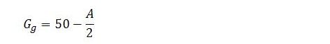
Here, A is total autonomous expenditure, including autonomous government spending. That is, A = C0 + I0 + G0 = A’ + G0.
Suppose, initially, that the level of autonomous government spending is 60 and private autonomous expenditure (A’ = C0 + I0) is 28. Putting A = 88 into the formula gives Gg = 6. Total government spending (G) will converge on G0 + Gg = 66.
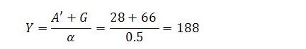
Making use of expression (5), full-employment output will converge on:
Using (6), the level of output produced in the broader economy will converge on:

Since average productivity in the broader economy is 2, employment in the broader economy converges on Lb = 92, with the remainder of employment (Lg = 8) in the job-guarantee program.
Job-guarantee output is:

With 8 percent of employment located in the job-guarantee sector, there is plenty of room for government to lift its autonomous spending. The multiplier effects of this will result in an expansion of activity in the broader economy and a contraction in job-guarantee employment and production.
For instance, if autonomous government expenditure were increased by 6 to G0 = 66, feedback between the broader economy and job-guarantee sector would result in a reduction in job-guarantee spending of 3 to Gg = 3 and an increase in total government spending of 3 to G = 69. Total output would rise to Y = 194. Job-guarantee output would contract from 4 to 2 and output in the broader economy would increase from 184 to 192. Employment in the broader economy would increase to 96, whereas employment in the job-guarantee sector would contract to 4.
An illustration of convergence
Understanding might also be enhanced by looking at the first part of the previous example in a different way. We can think in steps from initial autonomous acts of spending through to their multiplier effects, the automatic response of endogenous government spending, and the subsequent feedback between the broader economy and job-guarantee sector.
The sequence begins with government, firms and households autonomously spending 88, of which 60 is autonomous government spending. If it were not for the job guarantee, the expenditure multiplier (1/α) would be 2 and the full effect of the autonomous expenditure would be felt in the broader economy. So, the autonomous spending of 88 would notionally result in output of 176 in the broader economy. Since average productivity in the broader economy is assumed to be 2, this 176 of output would correspond to employment of 88. But, of course, there is a job guarantee. Employment of 88 in the broader economy would mean employment of 12 in the job-guarantee program because of our assumption that workers, through their labor-supply decisions, determine full employment to be employment of 100. Notionally, this would imply an amount of government spending on job-guarantee production of 12wL/ϕ = 9 (since we set wL to 1/2 and ϕ to 2/3).
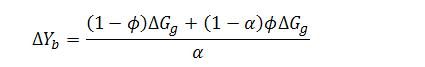
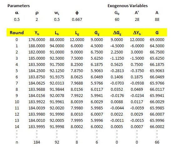
But this endogenous government spending of 9 would result in further demand for output produced in the broader economy. Of the 9 spent by government on the job-guarantee program in the initial stage (row zero in the table below), one-third (equal to 1 – ϕ) will immediately enter the broader economy. The other two-thirds (the fraction ϕ) will be received as wages by job-guarantee workers. As already discussed, the multiplier on this spending applicable to the broader economy is 1/α – ϕ, which in the current example equals 1.33. As a result, the change in income that would result from the initial job-guarantee expenditure of 9 will be 12. This is shown in the column labeled ΔYb. The change is entered in row 0 because the basis for its calculation is in that row. But the change in income registers in the following round of the process (round 1), as can be seen in the column labeled Yb.
In round 1 (the second row), the endogenous government expenditure of 9 has caused an expansion of employment in the broader economy and a contraction in the job-guarantee sector. This results in a reduction in endogenous government expenditure, which halves from 9 to 4.5. This negative change sets off a negative multiplier effect on the broader economy, with the relevant multiplier once again 1.33.
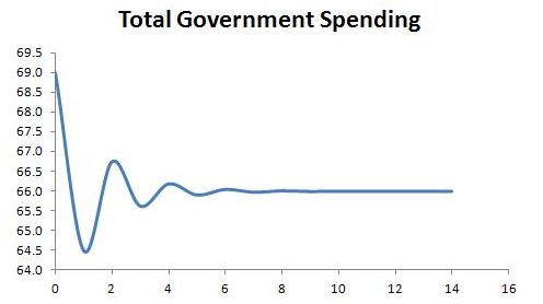
The table summarizes the feedback effects and illustrates the convergence of total government spending to G = 66, endogenous government spending to Gg = 6 and other endogenous variables to their respective values.
The convergence of total government spending to G = 66 and job-guarantee employment to Lg = 8 can also be represented graphically.