
We have seen that the ‘income-expenditure model’ combines key macro identities (introduced in parts 7 and 15) with particular behavioral assumptions to provide a theory of income determination (considered in parts 16 and 18). The behavioral assumptions relate to causation. The causation envisaged in the income-expenditure model has implications for the sectoral balances, some of which are the focus of the present post.
Recall that total leakages must equal total injections:
S + T = G + I
In a closed economy, the leakages are saving (S) and taxes (T). The injections are government spending (G) and private investment (I).
If we take all variables to the left-hand side and group them appropriately, we have:
(S – I) + (T – G) = 0
Or, in words:
Non-Government Balance + Government Balance = 0
As it stands, this is just an identity. But we can apply the behavioral assumptions of the income-expenditure model to consider various scenarios.
To do this, it will be helpful to derive a saving function by making use of the definition that saving is disposable income minus private consumption. In part 18 we defined tax and consumption functions:
T = tY
CP = C0 + c(Y – tY) = C0 + cY – ctY
Plugging these into our definition of saving (S = Y – T – CP) and rearranging enables us to express planned saving as a function of income:
S = Y – tY – (C0 + cY – ctY)
Upon rearrangement, and noting that the marginal propensity to save equals one minus the marginal propensity to consume (that is, s = 1 – c):
S = s(1 – t)Y – C0
The saving function enables us to consider the effects of changes in income on the non-government financial balance (NGB = S – I):
NGB = s(1 – t)Y – C0 – I
Likewise, we can consider the effects of changes in income on the government balance (GB) by taking account of the impact on tax revenue (using our definition T = tY).
GB = tY – G
We can consider an example by putting some numbers to the various parameters and exogenous variables. The parameters of the model are the marginal propensities to consume, tax and save. The exogenous variables are the components of spending that are autonomous of income, namely government spending, private investment and autonomous private consumption.
Let’s suppose, initially, that c = 0.8, t = 0.25 and s = 1 – c = 0.2. Using the formula for the multiplier:
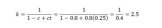
The value of the marginal propensity to leak (α = 1 – c + ct) says that forty percent (or 0.4) of extra income will leak to taxes and saving. The other sixty percent will go to induced private consumption. The value of the expenditure multiplier says that a given increase in autonomous spending (A) will cause total income to rise by two-and-a-half times the change in A.
Suppose, initially, that government spending (G) is 25, private investment (I) is 10 and autonomous private consumption (C0) is 5. We know from previous parts of the series that the economy will tend to converge to a level of output determined by the size of the expenditure multiplier (2.5) and the sum of autonomous expenditures (A = C + I + G = 40):
Y = kA = 2.5(40) = 100
With this information, we can work out the corresponding sectoral financial balances:
NGB = s(1 – t)Y – C0 – I = 0.2(1 – 0.25)(100) – 5 – 10 = 0
GB = tY – G = 0.25(100) – 25 = 0
Both sectors happen to have a zero balance. Non-government is spending an amount equal to its disposable income. Government is taxing out of the economy the same amount it is spending into it.
This is the initial situation. If anything happens to a parameter or exogenous variable, the above outcomes will be modified. In the remainder of this post, we consider a number of scenarios. At the start of each scenario we assume the initial situation described above. That is, changes in one scenario do not carry over to the next scenario. We re-set each time. For convenience of reference, here is a summary of the initial situation:
G = 25, I = 10, C0 = 5, c = 0.8, t = 0.25, s = 0.2
This means that:
A = 40, α = 0.4, k = 1/α = 2.5, Y = kA = 100
and
NGB = 0 = GB
Increase in private investment. Starting from the initial situation, suppose that private investment doubles from 10 to 20, with no other changes to the exogenous variables or parameters. This will cause income to rise by two-and-a-half times the rise in private investment. The higher income will result in more taxes and saving (though not as much extra saving as private investment). The overall effect will be for the government to move into surplus and the non-government into deficit. The results are shown below:
ΔY = k.ΔA = 2.5(10) = 25
Y = kA = 2.5(50) = 125
NGB = s(1 – t)Y – C0 – I = 0.2(1 – 0.25)(125) – 5 – 20 = -6.25
GB = tY – G = 0.25(125) – 25 = 6.25
The increase in private investment pushes non-government into deficit because the higher income does not leak only to saving, but also to taxes.
Increase in government spending. Starting again from the initial situation, suppose government spending increases by 10 (to 35), with no other exogenous changes. This will cause income, taxes and saving to rise. However, taxes will not rise by as much as government spending because some of the leakage will go to saving rather than taxes. The change in income and the new level of income will be the same as in the previous example. The sectoral balances become:
NGB = s(1 – t)Y – C0 – I = 0.2(1 – 0.25)(125) – 5 – 10 = 3.75
GB = tY – G = 0.25(125) – 35 = -3.75
The government balance has moved into deficit, enabling non-government to maintain a financial surplus over the period. The higher income has enabled more saving.
A higher rate of taxation. Again starting from the initial situation, suppose now that the marginal propensity to tax is increased from 0.25 up to 0.375. The effect of this will be to increase the marginal propensity to leak (α) from 0.4 to 0.5. This shrinks the expenditure multiplier (k) from 2.5 down to 2. The autonomous spending of A = 40 now tends to generate, via the multiplier process, a level of income of only Y = kA = 80. This has ramifications for the sectoral financial balances:
NGB = s(1 – t)Y – C0 – I = 0.2(1 – 0.375)(80) – 5 – 10 = -5
GB = tY – G = 0.375(80) – 25 = 5
The higher tax rates cause the government balance to move into surplus and weaken the economy, which is now generating lower income. Non-government is pushed into financial deficit because the weaker income and higher taxes impact negatively on saving. Note that since total injections have not changed, total leakages also remain the same. It is just that more of the leakage goes to taxes rather than saving as a result of the policy change.
A higher marginal propensity to save. Reverting one more time to the initial situation in which income is 100 and the multiplier is 2.5, suppose the marginal propensity to save is increased from one-fifth to one-third. This will cause the marginal propensity to leak (α) to increase from 0.4 to 0.5 and the multiplier (k) to shrink from 2.5 to 2. Income will tend to fall from 100 to 80 and the sectoral financial balances will once again be affected:
NGB = s(1 – t)Y – C0 – I = 0.33(1 – 0.25)(80) – 5 – 10 = 5
GB = tY – G = 0.25(80) – 25 = -5
This time it is the government that moves into deficit and the non-government that moves into financial surplus. Total leakages are the same as in the initial situation (total leakage is 35 in each case, equal to total injections). Saving has increased from 10 to 15 whereas taxes have fallen from 25 to 20. The reduction in income hits both taxes and saving, but households are now saving a higher fraction of a lower income.
