
The first section of the previous post outlined basic steady state relationships in a simplified economy with a job guarantee. There are various ways of expressing the same relationships that shed light on what is going on in the model. Here, a few ways of thinking about the levels of total income and job guarantee spending are noted.
Two reference points
The presentation in the previous post was guided by a desire to have all key expressions share the same denominator. The common denominator was α + q, where α is the marginal propensity to leak to taxes, saving and imports and q is the ratio of job guarantee spending to the income gap.
In thinking about an economy with a job guarantee, there are a couple of obvious reference points. One is the maximum possible level of income given the labor-supply choices of workers. This is the level of income that could notionally be generated if all employment happened to be in sector b (the broader economy) since productivity in that sector is assumed to be higher than in sector j (the job guarantee sector). In reality, Ymax would not be tolerated by policymakers because of the inflationary pressures likely to emerge. To the extent that some employment must be located in sector j, income will fall short of Ymax, leaving an income gap.
Another reference point is the level of income that would be generated in the absence of a job guarantee. This is equal to A / α, where A is autonomous demand.
In short, there is a maximum possible income (reference point 1), the income that would be generated in the absence of a job guarantee (reference point 2), and income itself. Income will be at a level somewhere between the two reference points whenever an income gap exists.
The following way of expressing the steady state level of income makes this clear:
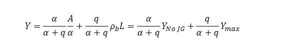
Here, ρb is sector b productivity and L is total employment. For now, both are taken to be exogenous. The expression depicts the level of income as a weighted average of the two reference levels, with the weights depending on the parameters α and q.
Job guarantee spending can be considered in a similar way:

This shows job guarantee spending as a fraction of the income that notionally could be generated beyond YNo JG. Again the parameters α and q shape the relationship in question.
The reference points can also be considered in terms of employment:

In this expression, ϕ is the fraction of job guarantee spending going to wages and wj the job guarantee wage. Both are exogenous. The expression says that job guarantee spending is just sufficient to generate the amount of employment L – LNo JG. Part of this employment is generated directly in sector j and part is generated indirectly through the multiplier impact of job guarantee spending on sector b income and employment.
Alternative way of obtaining the steady state relationships
The previous post discussed the notion of an income gap (or Ygap) that represents the difference between Ymax and income Y. It was observed that job guarantee spending can be thought of as a fraction q of the income gap. This suggests a different way of arriving at the steady state relationships.
The steady state condition and demand function are reproduced below.

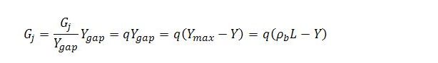
If job guarantee spending is regarded as a fraction of the income gap, then
Substituting this expression for Gj into the demand function and solving for steady state income gives the same expression for Y as presented in the previous post:
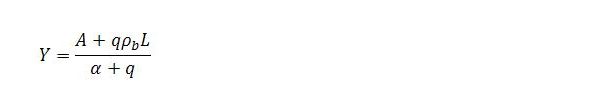
This expression can be substituted into the preceding one for Gj to get the steady state level of job guarantee spending and then the expressions for Y and Gj used to obtain the other relationships.
This might seem simpler than the approach adopted previously, but the make-up of q is left vague. The relevant expression for q can be obtained by noting that the income gap will be equal to the productivity differential (where wj is taken to define sector j productivity) multiplied by the level of sector j employment:

Since Gj = qYgap,

Solving for q:
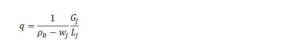
Noting that job guarantee spending per unit of sector j employment is wj / ϕ, we have

which matches the definition for q given in the previous post.
In the end, this method does not really save effort. But perhaps it offers a somewhat different perspective on the various relationships.
